eSTZwritR is available only on github. It can be
installed using the remotes or devtools
packages. Users from different operating systems (e.g. Mac and Windows)
have differing success with the above two packages in general. If one
package is not easy for the install, perhaps try the other.
# install.packages('devtools')
devtools::install_github('sagesteppe/eSTZwritR')

#install.packages('remotes')
#remotes::install_github('sagesteppe/eSTZwritR')
We will also load the core tidyverse packages for assorted data handling tasks.
Here we will load in the example data we will use for all steps of the vignette. These data are from Johnson, R. C., E. A. Leger, and Ken Vance-Borland. “Genecology of Thurber’s Needlegrass (Achnatherum thurberianum (Piper) Barkworth) in the Western United States.” Rangeland Ecology & Management 70.4 (2017): 509-517. They represent a rather complex eSTZ, composed of many polygons.
acth7 <- sf::st_read(file.path(
   system.file(package="eSTZwritR"), "extdata", 'ACTH7.gpkg')
)
Reading layer `ACTH7' from data source
  `/home/runner/work/_temp/Library/eSTZwritR/extdata/ACTH7.gpkg'
  using driver `GPKG'
Simple feature collection with 4967 features and 4 fields
Geometry type: MULTIPOLYGON
Dimension:     XY
Bounding box:  xmin: -121.5447 ymin: 36.53208 xmax: -111.0114 ymax: 46.35708
Geodetic CRS:  WGS 84
We will perform a few minor alteration on this data set which you may find useful in your own workflow. They are documented inline, understanding these operations is tangential to the rest of the vignette.
# This step was already run during creation of the package. simple feature
# geometries have certain rules about what constitutes a valid geometry. One
# of the most important rules (or at least the most violated) is that a polygon
# should not cross itself. We can easily fix that and several other types of
# errors using sf::st_make_valid() - this should be a common part of any spatial
# analysts workflow.
acth7 <- sf::st_make_valid(acth7)

# We also want to ensure that spatially contiguous polygons of the same seed zone
# are merged. This allows for more accurate assessments of the area covered by
# each seed zone in traditional data.frame/tibble type calculations. It also
# allows us to provide a unique ID to each polygon.

polygonsStart <- nrow(acth7)
acth7 <- acth7 |>
  # first we define a grouping variable, all polygons from these levels will be combined
  group_by(zone) |>
  # now we union (or dissolve) all polygons by the levels specified above, into
  # one multipolygon object per level.
  summarise(geom = st_union(geom)) |>
  # now we split apart the multipolygon into contiguous pieces.
  st_cast('POLYGON') |>
  # just making sure everything goes OK.
  st_make_valid()
Warning in st_cast.sf(summarise(group_by(acth7, zone), geom = st_union(geom)),
: repeating attributes for all sub-geometries for which they may not be
constant

polygonsEnd <- nrow(acth7)
message('\nThis data set now has: ', polygonsStart - polygonsEnd, ' fewer polygons')

This data set now has: 1587 fewer polygons

# You'll notice we lost some info!
# We lost columns containing the GRIDCODE - this is from when the data were converted
# from raster, area_ha, and ID for each polygon. The area_ha can be recalculated,
# and we can create new ID's for the polygons. We could use a left join to get the
# GRIDCODE back on. BUT take this is a lesson, some of these polygon geometry
# maintenance steps should be done early! Realistically before many analysis in
# the paper are done perhaps! We'll show you how to make some new IDs and
# calculate the areas again.

acth7 <- mutate(acth7, ID = 1:nrow(acth7), .before = 1)

# we can calculate the area like this
acth7 <- sf::st_transform(acth7, 5070) # we will put the data into an Equal area projection
# this type of projection minimizes the distortion of area.

# now we calculate the area using geodesic_areas (accounting for the curvature of the earth)
# we then convert the data into 'hectares' and will then drop some data attributes.
# see ?units for more info.
acth7 <- mutate(acth7, area_ha =
                  as.numeric(
                    units::set_units(
                      st_area(acth7), "hectare")), .before = geom)

# here we go! geodesic areas calculated from an equal area projection! This should
# be pretty well representative of how large each polygon is.

# now we will convert these data back to geographic coordinates system WGS84
acth7 <- sf::st_transform(acth7, 4326)

rm(polygonsStart, polygonsEnd)
Region Coding
The first step in using the package is determining which Department of Interior regions the data product is mostly associated with. The zones listed on the file will not be comprehensive, as we restrict the number of listed areas to two zones. However, they should give an OK indication of roughly the spatial extent which the data product covers.
rc <- regionCoding(acth7)
str(rc) # the returned data is a list of two objects, a vector and a data frame.
List of 2
 $ SuggestedName : chr "CGB-CPN"
 $ RegionsCovered:'data.frame': 3 obs. of  2 variables:
  ..$ REG_ABB: chr [1:3] "CGB" "CPN" "UCB"
  ..$ n      : int [1:3] 447 441 125

# Either format works to extract the data from the list.
rc$SuggestedName == rc[['SuggestedName']]
[1] TRUE
# I use this method (less typing), even though I like the look of the other method more...
rc$SuggestedName
[1] "CGB-CPN"
The SuggestedName vector contains the name which the
function proposes to use
We can look at the regions (well very small ones may be missed) which
our seed transfer zones is across by looking at the second item in our
list RegionsCovered.
knitr::kable(rc$RegionsCovered)| REG_ABB | n |
|---|---|
| CGB | 447 |
| CPN | 441 |
| UCB | 125 |
We see that we mostly cover the CBG region and CPN region, with some more coverage of the UCB region.
orderZones
The zones from a variety of data products have either no implicit ordering, or rather complex ordering. In these situations it can be difficult to determine which zones are in geographic and environmental proximity to each other. We have a function which users a very simple method to suggest an order for numbering the seed transfer zones in these instances. It will take a little bit of time to run, here we have the number of points used in calculating the order set to a low value, I encourage you to increase this value (to say 5000) when actually determining an order before distributing a data set.
oz <- orderZones(acth7, SeedZone = zone, n = 200)
# oz$Summary # i use kable so this looks nice online,
# just run oz$Summary to print to console.
knitr::kable(oz$Summary)| zone | SuggestedOrder | Zones_fct | MedianGAI | n |
|---|---|---|---|---|
| 12 | 1 | 12 | 0.1010 | 17 |
| 9 | 2 | 9 | 0.1274 | 5 |
| 11 | 3 | 11 | 0.1373 | 28 |
| 8 | 4 | 8 | 0.1606 | 78 |
| 4 | 5 | 4 | 0.1798 | 13 |
| 10 | 6 | 10 | 0.1937 | 4 |
| 7 | 7 | 7 | 0.1968 | 10 |
| 5 | 8 | 5 | 0.2087 | 35 |
| 2 | 9 | 2 | 0.2383 | 5 |
| 6 | 10 | 6 | 0.2760 | 5 |
Obviously, we can always get an order from the seed zones - but is there actually any merit to this order?
oz$PlotKruskal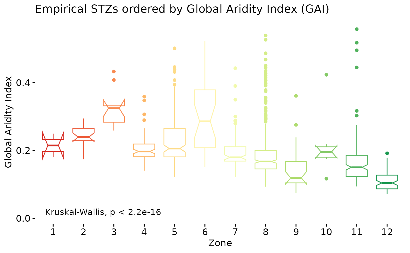
We can check that with the results from a Kruskal-Wallis test implemented using ggpubr. First visual impressions give an indication that a trend is present throughout the data, but that the differences between some groups appears negligible. So while a global trend exists, under a magnifying lens, relationships are more nuanced. In my opinion, the global trend is evidence enough, that using an ordering criterion like this is useful for simply trying to make some sense of categorical features. The results of the Kruskal-Wallis test (or one-way ANOVA on ranks) indicates that there is strong evidence that at least one group differs from the others, i.e. they were not drawn from the same distribution.
oz$PlotDunns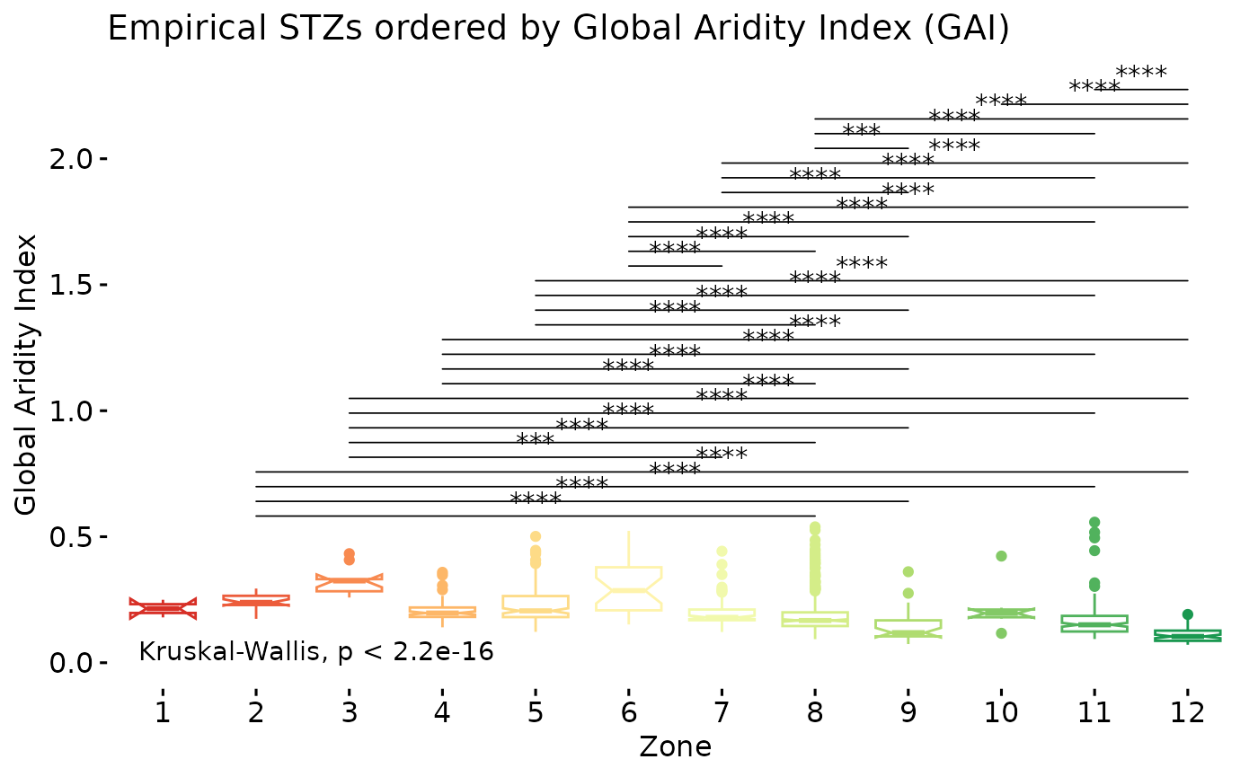
In this squished plot what we have depicted are the results from pairwise comparisons of all seed transfer zones using a Dunn’s test, with Holm’s p-adjustment method for multiple comparisons. If a line is missing between two groups, that indicates that a p-value of > 0.05 exists between the groups, showing little to no evidence of differences between them. The presence of the line indicates that a p-value beneath 0.05 is present, see ??stat_pwc for details on the coding. Our post-hoc test shows that the groups on either end of the aridity spectrum differ from each other. However, there is little evidence that the groups in the center of the spectrum differ from one another. Further there is no evidence that the more humid groups differ from one another.
To reiterate my initial impression from these plots, a continuum exists between the seed transfer zones. Some zones are markedly different from others, but most of them are able to run into each other.
Finally, we can make some maps and see how our seed zones differ on them - is their any intuitive sensibility here?
p1 <- ggplot(data = acth7, aes(fill = zone)) +
  geom_sf(color = NA) +
  theme_void() +
  scale_fill_distiller(palette = "RdYlGn", direction = 1) +
  labs(title = 'Original')

p2 <- ggplot(data = oz$Reclassified, aes(fill = zone)) +
  geom_sf(color = NA) +
  theme_void() +
  scale_fill_distiller(palette = "RdYlGn", direction = 1) +
  labs(title = 'Ordered')

p1 + p2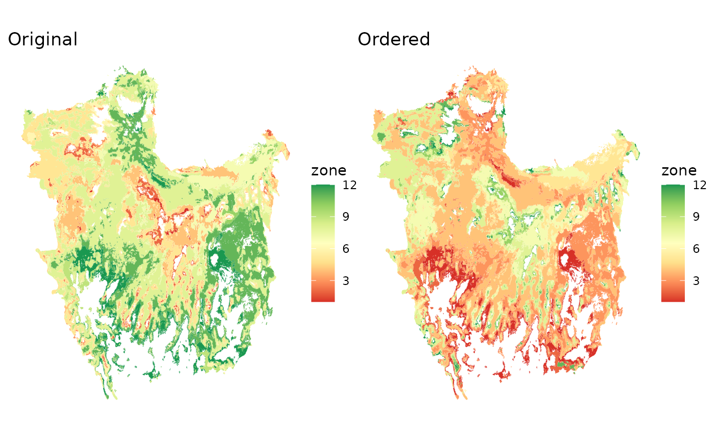
rm(p1, p2)The differences are not very loud, given the difficulty of interpreting habitat in the basin and range province, but they showcase a general trend from the more arid southern reaches, towards the more humid areas along the mountains of central Oregon. In lieu of a sensible and readily interpretable set of ordering to the data is this an improvement? In my mind yes, while others are free to disagree.
We can now apply these modifications to our input data, in fact, I’ll just overwrite out original ACTH7 variable with the output data from the function.
acth7 <- oz$ReclassifiedNote that this function uses Kruskal-Wallis tests by default, even though in this case we could probably swing an ANOVA due to the high number of groups, and high number of data points per group we were able to generate. This particular eSTZ example was chosen because it is a bit more complex than other products, and we don’t think swapping to an ANOVA in this function is warranted.
Vector Data Field Attibutes.
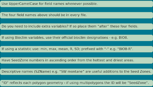
Many of these data products will be inspected and interacted with by human users, and they should cater to humans not just computers. One of the important decisions we can make to enhance this utility is to ‘order’ the fields in the spatial data, and to apply a consistent - and hence predictable - naming structure. The below image has four fields (ID, SeedZone, SZName, AreaAcres) which we consider mandatory for each file, and two supplementary fields which certain users may find useful (BIO1_R, BIO2_mean).
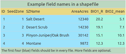
Some further guidance for naming and structuring shapefiles is provided below….
acth7_clean <- fieldsmakR(acth7, SeedZone = 'zone')
There is a column(s), `area_ha`, which we can't figure out the purpose of. It will be returned here, but FYI a list of bioclim variables is here: https://www.worldclim.org/data/bioclim.html. If you want to remove this/these columns this should do it: `dplyr::select(x, -c('area_ha'))`
head(acth7_clean)
Simple feature collection with 6 features and 5 fields
Geometry type: POLYGON
Dimension:     XY
Bounding box:  xmin: -118.4614 ymin: 38.99874 xmax: -111.828 ymax: 39.59041
Geodetic CRS:  WGS 84

[38;5;246m# A tibble: 6 × 6
[39m
     ID SeedZone SZName AreaAcres area_ha                               geometry

[3m
[38;5;246m<int>
[39m
[23m
[3m
[38;5;246m<int>
[39m
[23m
[3m
[38;5;246m<int>
[39m
[23m
[3m
[38;5;246m<dbl>
[39m
[23m
[3m
[38;5;246m<dbl>
[39m
[23m
[3m
[38;5;246m<POLYGON [°]>
[39m
[23m

[38;5;250m1
[39m     1        1      1
[4m4
[24m780.
[4m1
[24m935. ((-111.853 39.13208, -111.853 39.1237…

[38;5;250m2
[39m     2        1      1
[4m1
[24m
[4m7
[24m
[4m6
[24m473.
[4m7
[24m
[4m1
[24m416. ((-118.1864 39.41541, -118.178 39.415…

[38;5;250m3
[39m     3        1      1
[4m3
[24m298.
[4m1
[24m335. ((-116.003 39.07374, -116.003 39.0820…

[38;5;250m4
[39m     4        1      1
[4m1
[24m485.    601. ((-118.1614 39.02374, -118.1864 39.02…

[38;5;250m5
[39m     5        1      1
[4m1
[24m485.    601. ((-118.353 39.00708, -118.3614 39.007…

[38;5;250m6
[39m     6        1      1
[4m4
[24m
[4m2
[24m091.
[4m1
[24m
[4m7
[24m034. ((-113.1197 39.29874, -113.1197 39.30…
by default we try NOT to remove any columns, this way you don’t have to backtrack to recompute a variable. Please consider removing the column yourself, or rename it as necessary. I’ll re-familiarize you with this in a chunk further down.
We can also make the problem a little more difficult and see what the function returns
acth7_stuff <- acth7 |>
  dplyr::mutate(
    bio1_range = runif(n = dplyr::n()),
    bio12_avg = runif(n = dplyr::n()),
    bio9_m = runif(n = dplyr::n()),
  )

fieldsmakR(acth7_stuff, SeedZone = 'zone')
There is a column(s), `area_ha`, which we can't figure out the purpose of. It will be returned here, but FYI a list of bioclim variables is here: https://www.worldclim.org/data/bioclim.html. If you want to remove this/these columns this should do it: `dplyr::select(x, -c('area_ha'))`
Simple feature collection with 3380 features and 8 fields
Geometry type: POLYGON
Dimension:     XY
Bounding box:  xmin: -121.5447 ymin: 36.53208 xmax: -111.0114 ymax: 46.35708
Geodetic CRS:  WGS 84

[38;5;246m# A tibble: 3,380 × 9
[39m
      ID SeedZone SZName AreaAcres BIO1_R BIO9_m BIO12_mean area_ha

[3m
[38;5;246m<int>
[39m
[23m
[3m
[38;5;246m<int>
[39m
[23m
[3m
[38;5;246m<int>
[39m
[23m
[3m
[38;5;246m<dbl>
[39m
[23m
[3m
[38;5;246m<dbl>
[39m
[23m
[3m
[38;5;246m<dbl>
[39m
[23m
[3m
[38;5;246m<dbl>
[39m
[23m
[3m
[38;5;246m<dbl>
[39m
[23m

[38;5;250m 1
[39m     1        1      1
[4m4
[24m780. 0.058
[4m4
[24m 0.804       0.179
[4m1
[24m935.

[38;5;250m 2
[39m     2        1      1
[4m1
[24m
[4m7
[24m
[4m6
[24m473. 0.440  0.154       0.420
[4m7
[24m
[4m1
[24m416.

[38;5;250m 3
[39m     3        1      1
[4m3
[24m298. 0.224  0.893       0.537
[4m1
[24m335.

[38;5;250m 4
[39m     4        1      1
[4m1
[24m485. 0.955  0.871       0.253    601.

[38;5;250m 5
[39m     5        1      1
[4m1
[24m485. 0.148  0.859       0.430    601.

[38;5;250m 6
[39m     6        1      1
[4m4
[24m
[4m2
[24m091. 0.351  0.630       0.754
[4m1
[24m
[4m7
[24m034.

[38;5;250m 7
[39m     7        1      1
[4m1
[24m318. 0.570  0.396       0.356    533.

[38;5;250m 8
[39m     8        1      1
[4m1
[24m317. 0.033
[4m4
[24m 0.551       0.936    533.

[38;5;250m 9
[39m     9        1      1
[4m6
[24m916. 0.461  0.433       0.634
[4m2
[24m799.

[38;5;250m10
[39m    10        1      1
[4m1
[24m484. 0.534  0.077
[4m5
[24m      0.605    600.

[38;5;246m# ℹ 3,370 more rows
[39m

[38;5;246m# ℹ 1 more variable: geometry <POLYGON [°]>
[39m
See that the function can make some modifications to very simple abbreviations which we anticipate exist in the wild (range -> R, avg -> mean), but we cannot do much with BIO9_m, because we do not know what to do with it - should it be mean? max? min?
Please further note the function will not emit a warning if a BIO column is unrecognized, so please refer to the rules above and your output to determine if you need to manually alter any values so they are readily interpretable to other users.
rm(acth7_stuff, acth7)Directory (Folder) Structure & File Naming
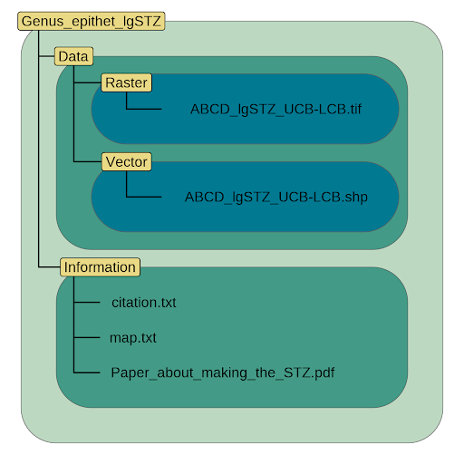
dirmakR(
  outpath = '~/Documents/EmpiricalSeedZones',
  sci_name = 'Eriocoma_thurberiana',
  x = acth7_clean,
  regioncode = rc,
  nrcs_code = 'ACHT7',
  estz_type = 'cg',
  overwrite = TRUE
)
Maps
Maps can oftentimes be used in lieu of the actual spatial data
product itself for many applications. We also use them frequently to
verify that values are ‘mapped’ over correctly in GIS, a problem which
should now be alleviated with more defined field naming conventions. The
maps which eSTZwritR makes are meant to be, well are, full
page PDFs in either a landscape or portrait orientation. We will also
return a map to the R plot pane, but that is a much smaller format than
the map is intended to be used at. So when you are actually using the
function, focus on only altering maps if the appearance of the PDF’s
leave something to be desired, not the examples from the viewing
pane.
map <- mapmakR(
  acth7_clean,
  sci_name = 'Eriocoma thurberiana', # this will become the title.
  save = FALSE, # whether to write to disk, defaults to TRUE
  landscape = FALSE, # defaults ot TRUE, we want a landscape page
  ecoregions = TRUE, # whether to add unlabeled L4 ecoregions or not.
  cities = TRUE, # whether to add some cities to the map
  caption =
    'Data from Johnson et al. 2017. https://doi.org/10.1016/j.rama.2017.01.004'
  # Cite where the data comes from!!! A doi would be great too ;-) !
)
The code to save the map is simple and below, we let one of our
arguments revert to it’s boolean defaults (save == TRUE), and supply an
output directory outdir to save our map too. Note that
all ancillary information for our projects go into the
Information sub-directory.
mapmakR(acth7_clean,
  species = 'Eriocoma thurberiana', # this will become the title.
  save = FALSE,
  outdir = '~/Documents/EmpiricalSeedZones/Eriocoma_thurberianacgSTZ/Information',
  landscape = FALSE, # defaults ot TRUE, we want a landscape page
  caption =
    'Data from Johnson et al. 2017. https://doi.org/10.1016/j.rama.2017.01.004'
  # Cite where the data comes from!!! A doi would be great too ;-) !
)
Here is a call to have it show up in the viewing pane, definitely do not judge them from this format. Save a copy locally before scrutinizing them, all it takes to do that is to change ‘save = FALSE’ to TRUE in the code chunk above.
mapWe show the saved PDF version of the map below. It is definitely a very strange format to view it in, but the only way I can figure out how to get it loaded into this vignette and pass the R package checks. On firefox, at least, you can download the map from this viewer if you want to be able to zoom in on it.
Pre-rendered PDF map of eSTZ
Bonus Activity - Naming the Seed Zones!
One suggestion within a paper we published stemming from this project is that all individual eSTZs seed zones should have a colloquial name for communicating them broadly. As individuals we generally find it easier to remember phrases, than simply numbers, even if they are ordered by an aridity gradient.
This section will be slightly wonky, I am going to open up the cleaned set of vector data we have created in a common Geographic Information System (GIS) with a Graphical User Interface (GUI). While there are several good GIS with GUI, we will ues the one I recommend every single time, QGIS. QGIS is totally free, works on essentially all operating systems and most flavours of linux, and is kind of like what ESRI products would be like if they weren’t terrible. If you want to download QGIS feel free to do so, it’s available here, but othewise you can just read the text and you’ll get an idea of what I mean by seed zone names.
data.frame(
  SeedZone = 1:12,
  SZName = c('Arid Valley Bottoms', 'Arid Valleys',  'Central Valleys',
             'Plains', 'North/Eastern Plains', 'Northern Alluvial Fans/Slopes',
             'Sagebrush Steppe (lower)', 'Sagebrush Steppe (mid)', 'Sagebrush Steppe (upper)',
             'Mountain (lower)', 'Moutain (mid)', 'Mountain (high)'
             )
)
   SeedZone                        SZName
1         1           Arid Valley Bottoms
2         2                  Arid Valleys
3         3               Central Valleys
4         4                        Plains
5         5          North/Eastern Plains
6         6 Northern Alluvial Fans/Slopes
7         7      Sagebrush Steppe (lower)
8         8        Sagebrush Steppe (mid)
9         9      Sagebrush Steppe (upper)
10       10              Mountain (lower)
11       11                 Moutain (mid)
12       12               Mountain (high)