Custom Label Templates
custom_label_templates.RmdOverview
Obviously, everyone wants to be able to customize their label
templates! Why go through the bother of installing and running
BarnebyLives if you cannot do that! So here are a couple
examples of tweaking around with the default skeleton to get some labels
which will… Look familiar.
Note that the labels are made using LaTeX, an awesome guide for LaTeX (relevant to the level you will be using it at) is Overleaf.org, and check the links in the side bar too!
In this vignette, I will show you what the three default templates look like, and then we will make some slight customizations to them.
Examples
As a reminder, the standard template (skeleton.Rmd)
looks like this.
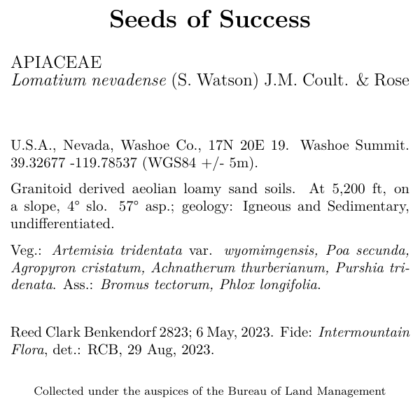
Another included template, for the Seeds of Success program
(skeletonSOS.Rmd), looks like this. Seeds of Success is a
rad program all about how plant science will save the planet. This
collection didn’t lead to a collection, but I am largely indebted to it
for a ton of testing data from a whole slew of collectors (holla @
Chicago Botanic Garden & University of Nevada Reno too!)
And our final default template (skeleton-new.Rmd) looks
like this
Modifications
library(BarnebyLives)
library(tidyverse)

local <- file.path('~', 'Documents', 'assoRted', 'Barneby_Lives_dev', 'LabelStyles')

l.nevadense <- collection_examples |>
  filter(Collection_number == 2823)

write.csv(l.nevadense, file.path(local, 'SoS-ExampleCollection.csv'))
All of the labels can be copied from their original locations using the following code.
p2lib <- file.path(
  system.file(package = 'BarnebyLives'),
  'rmarkdown', 'templates', 'labels', 'skeleton'
  )

# here we copy over one of the skeletons which we are going to modify in this example
file.copy(
  from = file.path(p2lib, 'SoS-skeleton.Rmd'),
  to = file.path(local, 'SoS-skeleton.Rmd')
  )

rm(p2lib)
When using the program you will need to copy a template from it’s location within the package to a ‘local’ location. This is because you will always need to modify a small part of the skeleton which defines where the document should look for your data it will put on the labels, see the ‘creating_labels’ vignette for details. Any changes you make to the skeleton’s in the package directory will be lost anytime you update the package. Once the file is in that location it can easily be opened for safe editing. So by ‘local’ I basically mean put the file in a location on your computer which will not be overwritten when you update the package, which may happen without your knowledge if this becomes a dependency to another package (which seems highly unlikely to me). Obviously it’s good to try and place all of these skeletons in the same location so you don’t have to do much hunting around to find them, the ‘spaces’ in LaTeX formatting can make things go haywire quick, so it’s nice to have a backup version as you are tailoring a version.
While I am about to be very busy for the next few years I am happy to
accept pull requests so that BL has a greater variety of herbarium
templates, likewise you can make your own writer_* type
functions and push those to the package. If you have questions about how
to do this, many good github resources/guides exist, and i am happy to
try and help with incorporating materials.
One final note is that LaTeX uses spaces, or ’ ’ for controlling content. In particular two spaces will force the text onto a new line. It is hard for me illustrate these in the examples, but I’ll try and do my best to mention them when relevant.
For this example we will focus on the final default template, which is a pretty middle of the road design.
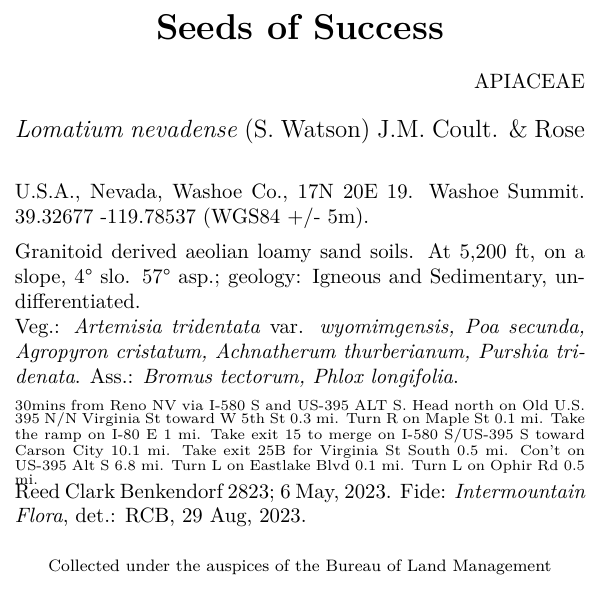
Hmm that’s a busy label, we could try and reduce the directions manually… Or, we can just rid of them! Around line 50 we can just remove the following details.
Delete this!
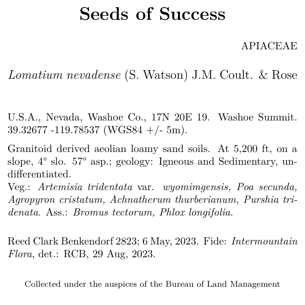
That looks better! But now that we can, I want to open up some space between the habitat notes and vegetation information. It’s simple, all we need is to empty a blank line to the document
\begingroup
`r data$Gen`. `r writer(data$Site)` `r data$latitude_dd` `r data$longitude_dd` (`r data$Datum` `r writer(data$Coordinate_Uncertainty)`).

`r writer(data$Habitat)`. `r data$physical_environ`
Veg.: `r species_font(data$Vegetation)` `r associates_writer(data$Associates)`
`r writer(data$Notes)`
\endgroup
Can become the chunk below. All we do is enter a blank line between ‘r writer()…’ and ‘Veg.’
\begingroup
`r data$Gen`. `r writer(data$Site)` `r data$latitude_dd` `r data$longitude_dd` (`r data$Datum` `r writer(data$Coordinate_Uncertainty)`).

`r writer(data$Habitat)`. `r data$physical_environ`

Veg.: `r species_font(data$Vegetation)` `r associates_writer(data$Associates)`
`r writer(data$Notes)`
\endgroup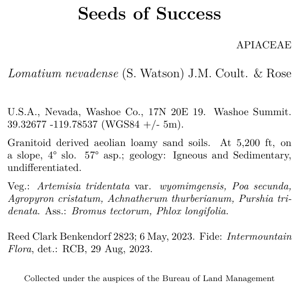
That’s better!
“All I want is to breathe I’m too thin”
“Won’t you breathe with me?”
“Find a little space, so we can move in-between In-Between it”
“And keep one step ahead, of yourself.”
Now let’s change the line that controls the size of the font for the
project name. Here we will be making the font size smaller by shifting
from the LARGE to the large argument.
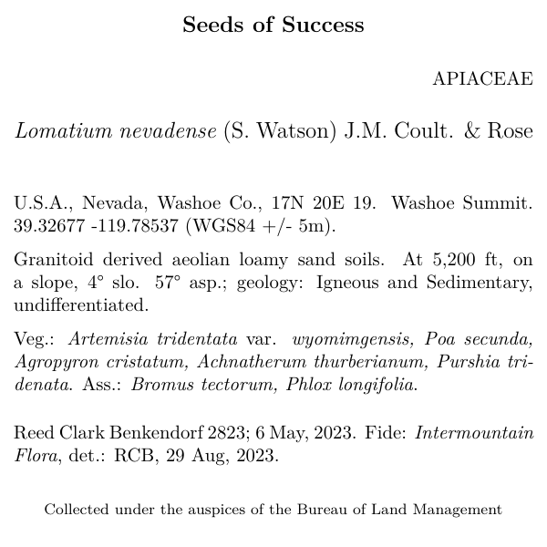
Here we change the location of the family on the label (currently
aligned right). Let’s make the family left aligned.
Note that all calls to R are in a single set of smart quotes, and ‘R’,
this allows us to run R commands without having to create a code chunk
for them in the more common markdown syntax. We have created a few
commands which help format the writing output for making the labels like
nice.
\begin{flushright}
\uppercase{`r data$Family`}
\end{flushright}

\begingroup
\large
`r writer(paste(data$Genus, data$Epithet), italics = TRUE)` `r writer(data$Binomial_authority)` `r writer(data$Infrarank)` `r  writer(data$Infraspecies, italics = TRUE)` `r writer(data$Infraspecific_authority)`
\endgroup
\normalsize
If you remove the flushright commands you basically end
up with this:
\large
\uppercase{`r data$Family`}
\begingroup
`r writer(paste(data$Genus, data$Epithet), italics = TRUE)` `r writer(data$Binomial_authority)` `r writer(data$Infrarank)` `r  writer(data$Infraspecies, italics = TRUE)` `r writer(data$Infraspecific_authority)`
\endgroup
\normalsize
This requires us to delete the first three lines while we copy the family down into the ‘group’. Which brings up a good point, these ‘groups’ are used to more or less create elements held together like paragraphs. If we had omitted to bring family into the group, there would be a smidge more space between it and the scientific name (as exemplified with the habitat and vegetation alterations.)
We may also decide that we want to put determination information
right under the species. We can do that by just moving these elements
around. (Be sure to delete the call to writer_fide from the
chunk located all the way near the bottom of the skeleton!).
And bring it up to where the scientific name is printed, and make the font for the det info smaller.
\begingroup
\large
`r writer(paste(data$Genus, data$Epithet), italics = TRUE)` `r writer(data$Binomial_authority)` `r writer(data$Infrarank)` `r  writer(data$Infraspecies, italics = TRUE)` `r writer(data$Infraspecific_authority)`
\normalsize
`r writer_fide(data)`
\endgroup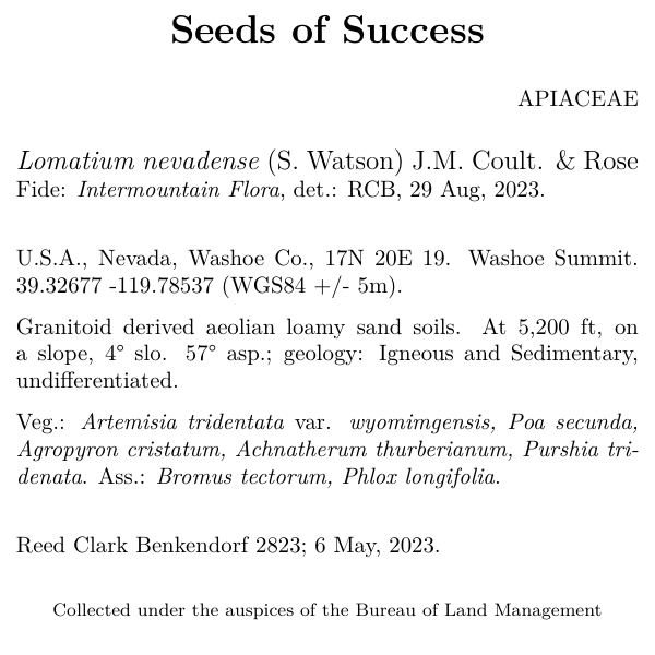
Obviously, the way I enter data for determination would be bad for this! using my initials after my full name makes sense, in this context, who the hell is “RCB” you would wonder? I am one in a sea of botanists named ‘Reed’, and certainly other - more illustrious - RCB’s are out there.
In summary
This is an odd vignette to create because it relies on multiple languages, especially one where ’ ’ spaces are very important. Just bear in mind you can make big changes to labels with small steps (maybe too small?)! The overleaf guide has https://www.overleaf.com/learn everything you need, and you’ll probably realize this pales in comparision.