Getting Started

This vignette showcases the different sampling designs applied to the same species.

set up

safeHavens can be installed directly from github.

# remotes::install_github('sagesteppe/safeHavens') 

library(safeHavens)
library(sf) ## vector operations
library(terra) ## raster operations
library(spData) ## basemap data
library(dplyr) ## general data handling
library(ggplot2) ## plotting 
library(patchwork) ## multiplots
set.seed(23) 

planar_proj <- "+proj=laea +lat_0=-15 +lon_0=-60 +x_0=0 +y_0=0 +datum=WGS84 +units=m +no_defs"

Defining a Species Range or Domain for Sampling

The core of safeHavens sampling schemes is the species range or domain. Curators can sample across the entire range or focus on a region, such as a country or ecoregion. Both approaches are supported. We show how to use occurrence data to define species ranges across various sampling schemes.

Below we will use sf to simply buffer occurrence points to create a species range across multiple South American nations.

x <- read.csv(file.path(system.file(package="dismo"), 'ex', 'bradypus.csv'))
x <- x[,c('lon', 'lat')]
x <- sf::st_as_sf(x, coords = c('lon', 'lat'), crs = 4326)
x_buff <- sf::st_transform(x, planar_proj) |>
  # we are working in planar metric coordinates, we are
  # buffer by this many / 1000 kilometers. 
  sf::st_buffer(125000) |> 
  sf::st_as_sfc() |> 
  sf::st_union()

plot(x_buff)

Alternatives include creating a convex hull for widespread species (see ‘Worked Example’) or masking a binary SDM surface as the domain (see below and ‘Species Distribution Model’).

Prep a base map

We will use the spData package which uses naturalearth for it’s world data and is suitable for creating maps at a variety of resolutions.

x_extra_buff <- sf::st_buffer(x_buff, 100000) |> # add a buffer to 'frame' the maps
  sf::st_transform(4326)

americas <- spData::world
americas <- sf::st_crop(americas, sf::st_bbox(x_extra_buff)) |>
  dplyr::select(name_long)
Warning: attribute variables are assumed to be spatially constant throughout
all geometries

bb <- sf::st_bbox(x_extra_buff)

map <- ggplot() + 
  geom_sf(data = americas) + 
  theme(
    legend.position = 'none', 
    panel.background = element_rect(fill = "aliceblue"), 
    panel.grid.minor.x = element_line(colour = "red", linetype = 3, linewidth  = 0.5), 
    axis.ticks=element_blank(),
    axis.text=element_blank(),
    plot.background=element_rect(colour="steelblue"),
    plot.margin=grid::unit(c(0,0,0,0),"cm"),
    axis.ticks.length = unit(0, "pt"))+ 
  coord_sf(xlim = c(bb[1], bb[3]), ylim = c(bb[2], bb[4]), expand = FALSE)

rm(x_extra_buff, americas)

Running the Various Sample Design Algorithms

Now that we have some data which can represent species ranges, we can run the various sampling approaches. The table in the introduction is reproduced here.

Function	Description	Comp.	Envi.
PointBasedSample	Creates points to make pieces over area	L	L
EqualAreaSample	Breaks area into similar size pieces	L	L
OpportunisticSample	Using PBS with existing records	L	L
KMedoidsBasedSample	Use ecoregions or STSz for sample	L	M
IBDBasedSample	Breaks species range into clusters	H	M
PolygonBasedSample	Using existing ecoregions to sample	L	H
EnvironmentalBasedSample	Uses correlations from SDM to sample	H	H

Note in this table ‘Comp.’ and ‘Envi.’ refer to computational and environmental complexity respectively, and range from low (L) through medium to high.

PointBasedSample

PointBasedSample selects a set of regularly spaced points across the domain and assigns each point’s cluster to the area nearest to it. This strictly spatial approach relies on even spacing as its main differentiator. It will work very well for common species without many gaps in their distributions.

pbs <- PointBasedSample(x_buff, reps = 50, BS.reps = 333)
pbs.sf <- pbs[['Geometry']]

pbs.p <- map + 
  geom_sf(data = pbs.sf, aes(fill = factor(ID))) + 
#  geom_sf_label(data = pbs.sf, aes(label = ID), alpha = 0.4) + 
  labs(title = 'Point') + 
  coord_sf(expand = F)

pbs.p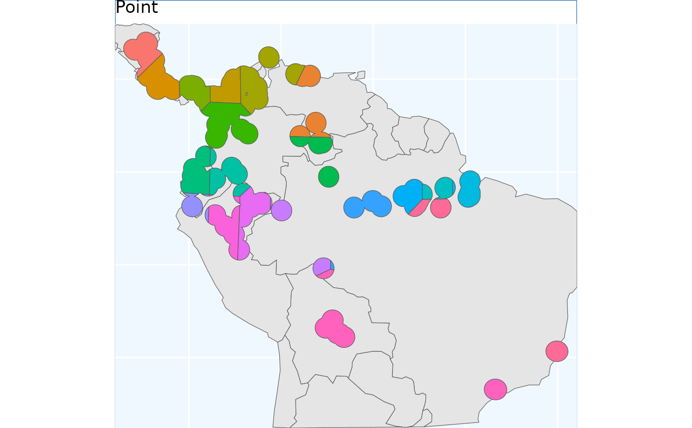

EqualAreaSample

Perhaps the simplest method offered in safeHavens is EqualAreaSample. It creates many points (pts, defaulting to 5000) within our target domain and subjects them to k-means clustering, where the groups are specified by n, our target number of collections. Points in each group are merged into polygons that fill the geographic space, intersected with the species’ range, and their areas are measured. This runs multiple times (default: 100 reps), and the set with the smallest variance in polygon size is selected

This process stands apart from point-based sampling: instead of growing clusters from a set of regular points, EqualAreaSample uses many input points and relies on area-balancing clustering. This allows for more equally sized regions.

eas <- EqualAreaSample(x_buff, planar_proj = planar_proj) 

eas.p <- map + 
  geom_sf(data = eas[['Geometry']], aes(fill = factor(ID))) + 
#  geom_sf_label(data = eas.sf, aes(label = ID), alpha = 0.4) + 
  labs(title = 'Equal Area') + 
  coord_sf(expand = F)
eas.p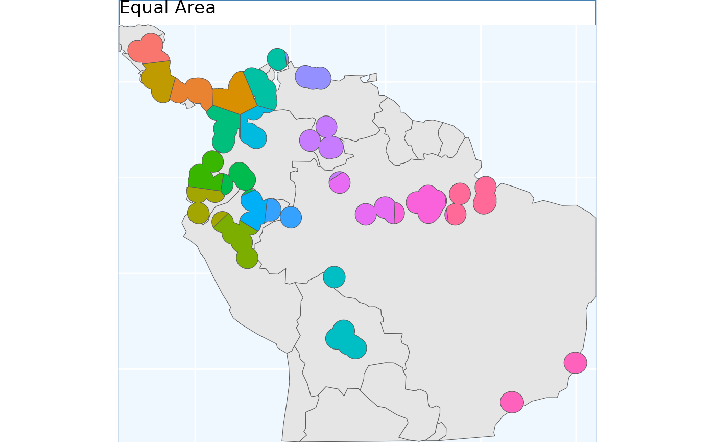

The results look quite similar to PointBasedSample.

OpportunisticSample

Users may be interested in how they can embed their existing collections into a sampling framework. The function OpportunisticSample makes a few minor modifications to the point-based sample and designs it around existing collections. It may not perform well if collections are close together, but, as the saying goes, “a bird in hand is worth two in the bush”. As we have observed, the previous sampling schemes have produced somewhat similar results, so we used the PointBasedSample as the framework for embedding in this function.

exist_pts <- sf::st_sample(x_buff, size = 10) |> 
   sf::st_as_sf() |> # ^^ randomly sampling 10 points in the species range
   dplyr::rename(geometry = x)

os <- OpportunisticSample(polygon = x_buff, n = 20, collections = exist_pts, reps = 50, BS.reps = 333)

os.p <- map + 
  geom_sf(data = os[['Geometry']], aes(fill = factor(ID))) + 
#  geom_sf_label(data = os.sf, aes(label = ID), alpha = 0.4) + 
  geom_sf(data = exist_pts, alpha = 0.4) + 
  labs(title = 'Opportunistic') + 
  coord_sf(expand = F)

os.p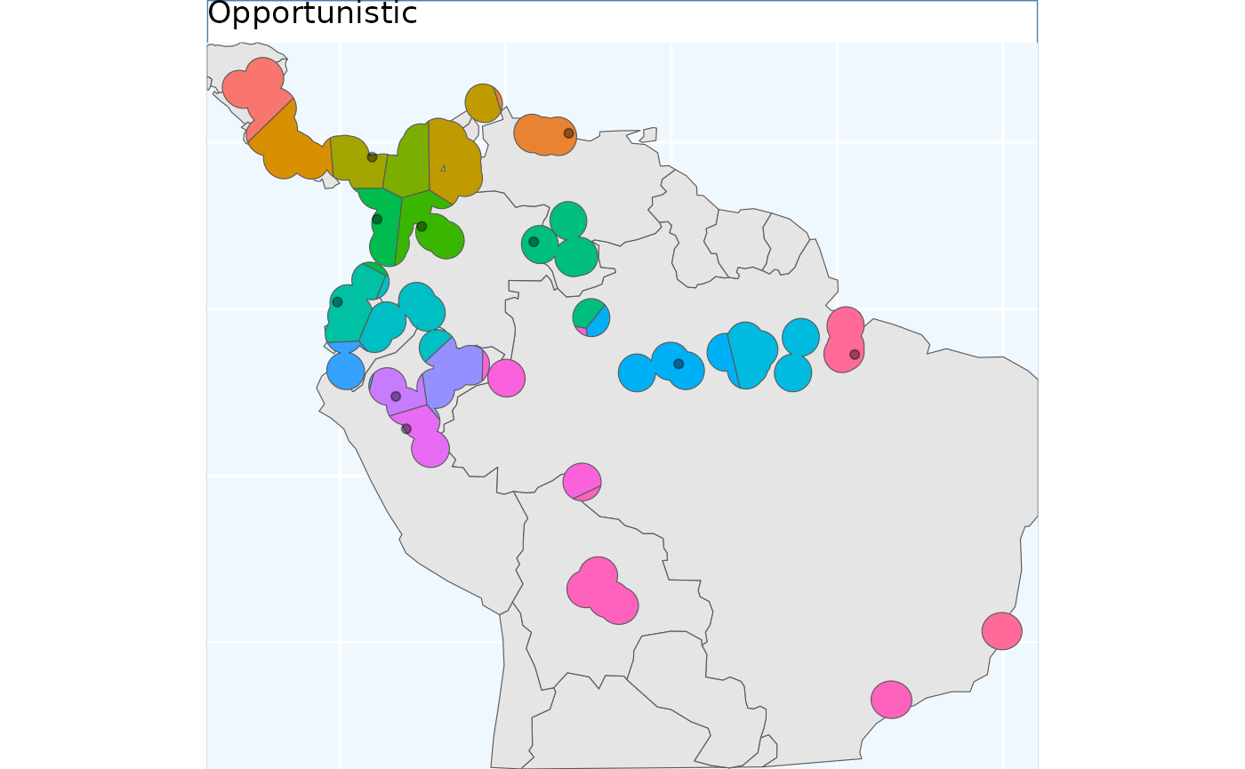

Here, the grids have been aligned around the existing collections. The results from this function can lead to some oddly shaped clusters, but a bird in hand is worth two in the bush.

Isolation by Distance Based Sample

Isolation by Distance is the fundamental idea behind this package. This function applies Isolation by Distance (IBD) without added parameters, creating clusters based solely on spatial genetic structure, not geographic spacing or area balancing, which distinguishes it from previous methods.

Note that this function requires a raster, rather than a vector, input. Here we can prepare the surface.

files <- list.files( 
  path = file.path(system.file(package="dismo"), 'ex'),
  pattern = 'grd',  full.names=TRUE ) 
predictors <- terra::rast(files) 

x_buff.sf <- sf::st_as_sf(x_buff) |> 
  dplyr::mutate(Range = 1) |> 
  sf::st_transform( terra::crs(predictors))

# and here we specify the field/column with our variable we want to become an attribute of our raster
v <- terra::rasterize(x_buff.sf, predictors, field = 'Range') 

Run the function here.

# now we run the function demanding 20 areas to make accessions from, 
ibdbs <- IBDBasedSample(
    x = v, 
    n = 20, 
    fixedClusters = TRUE, 
    template = predictors, 
    planar_proj = planar_proj
    )

And plot the results below.

ibdbs.p <- map + 
  geom_sf(data = ibdbs[['Geometry']], aes(fill = factor(ID))) + 
#  geom_sf_label(data = os.sf, aes(label = ID), alpha = 0.4) + 
  labs(title = 'IBDistance') + 
  coord_sf(expand = F)

[1m
[22mCoordinate system already present.

[36mℹ
[39m Adding new coordinate system, which will replace the existing one.

## for the sake of comparing areas below, we will intersect this to the same extents as the earlier surfaces. 
ibdbs_crop <- sf::st_intersection(ibdbs[['Geometry']], sf::st_union(x_buff.sf))
ibdbs.p2 <- map + 
  geom_sf(data = ibdbs_crop, aes(fill = factor(ID))) + 
#  geom_sf_label(data = os.sf, aes(label = ID), alpha = 0.4) + 
  labs(title = 'IBDistance') + 
  coord_sf(expand = F)

[1m
[22mCoordinate system already present.

[36mℹ
[39m Adding new coordinate system, which will replace the existing one.

ibdbs.p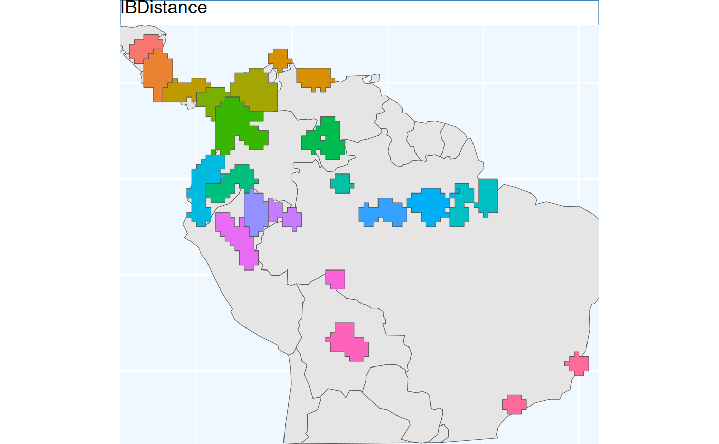

Because results are derived from rasters, clusters have straight lines and 90-degree corners. Despite the raster effects, cluster borders look more natural, and polygons align better with classes than previous methods.

Isolation by Resistance

This workflow requires a couple of steps. We have a dedicated vignette for Isolation by Resistance with full details. Here, we will just load the data you get when you run that vignette.

ibr <- sf::st_read(
  file.path(system.file(package="safeHavens"), 'extdata', 'IBR.gpkg'), 
  quiet = TRUE)

ibr.p <- map + 
  geom_sf(data = ibr, aes(fill = factor(ID))) +
  labs(title = 'IBResistance') + 
  coord_sf(expand = F)

[1m
[22mCoordinate system already present.

[36mℹ
[39m Adding new coordinate system, which will replace the existing one.

PolygonBasedSample

This method is widely used for native seed collection in North America. However, I am not sure exactly how practitioners implement it, or whether the application formats are consistent among practitioners! For these reasons, a few different sets of options are supported for a user.

For general usage, two parameters are always required x, which is the species range as an sf object, and ecoregions, the sf object containing the ecoregions of interest. The ecoregions file does not need to be subset to the range of x quite yet - the function will take care of that. Additional arguments to the function include, as usual, n, which specifies how many accessions we are looking for in our collection. Two additional arguments relate to whether we are using Omernik Level 4 ecoregions data or ecoregions (or biogeographic regions) from another source. These are OmernikEPA and ecoregion_col. If you are using the official EPA release of ecoregions, then both of these are optional. If you are not using the EPA product, then both should be supplied, but only the ecoregion_col argument is totally necessary. This column should contain the unique name of the highest-resolution ecoregion you want to use from the dataset. For many data sets, such as our example, we call ‘neo_eco’; this may be the only field with ecolevel information!

neo_eco <- sf::st_read(
  file.path(system.file(package="safeHavens"), 'extdata', 'NeoTropicsEcoregions.gpkg'), 
  quiet = TRUE) |>
  dplyr::rename(geometry = geom)

head(st_drop_geometry(neo_eco)[,c('Provincias', 'Dominio', 'Subregion')]) |>
  knitr::kable()

Provincias	Dominio	Subregion
Araucaria Forest province	Parana	Chacoan
Atacama province	NA	South American Transition Zone
Atlantic province	Parana	Chacoan
Bahama province	NA	Antillean
Balsas Basin province	Mesoamerican	Brazilian
Caatinga province	Chacoan	Chacoan

x_buff <- sf::st_transform(x_buff, sf::st_crs(neo_eco))
ebs.sf <- PolygonBasedSample(x_buff, zones = neo_eco, n = 20, zone_key = 'Provincias')

# crop it to the other objects for plotting
ebs.sf <- st_crop(ebs.sf, bb)

ebs.p <- map + 
  geom_sf(data = ebs.sf , aes(fill = factor(allocation))) + 
  labs(title = 'Ecoregion') + 
  coord_sf(expand = F)

This output differs from the others we will see; here, we have depicted the number of collections to be made per ecoregion. Because the number of ecoregions exceeds our requested sample size, the return object can only take on two values: no collections or one collection.

EnvironmentalBasedSample

The EnvironmentalBasedSample can only be used if you have species distribution model data. We have included the outputs of the vignette ‘Species Distribution Model’ with the package so they are available to this vignette.

load the SDM predictions

Here, we load the results of the sdm processing from the package data.

sdModel <- readRDS(
  file.path(system.file(package="safeHavens"), 'extdata',  'sdModel.rds')
  )

sdModel$RasterPredictions <- terra::unwrap(sdModel$RasterPredictions)
sdModel$Predictors <- terra::unwrap(sdModel$Predictors)
sdModel$PCNM <- terra::unwrap(sdModel$PCNM)

And load the threshold predictions

sdm <- terra::rast(
  file.path(system.file(package="safeHavens"), 'extdata',  'SDM_thresholds.tif')
  )
terra::plot(sdm)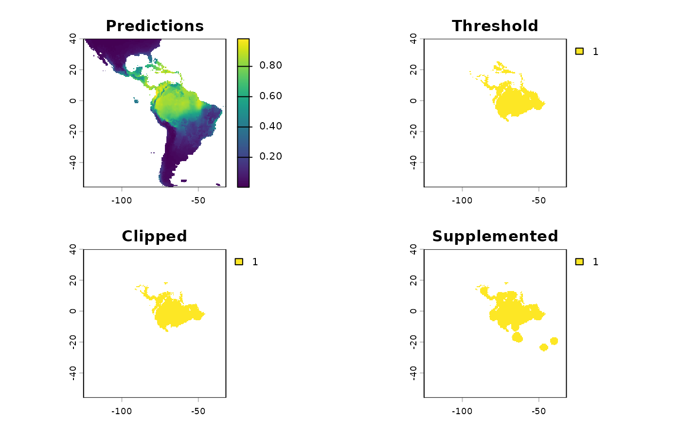

Once these data are loaded into R, we will scale the rasters (using RescaleRasters), which will serve as surfaces to predict from (this is also done above!), then we will run the algorithm (EnvironmentalBasedSample). However, before we run the algorithm, we will need to create a directory (also called a ‘folder’) on our computers to save the results from the function EnvironmentalBasedSample. Whereas earlier in this vignette we showcased that the functions generated the species distribution model, and us saving the results were a two-stage process (e.g. to create the SDM and associated products we used: elasticSDM, PostProcessSDM, and RescaleRasters, before finally saving relevant data with writeSDMresults), this function produces both the product and writes out ancillary data simultaneously. This approach was chosen as this function is only writing out four objects: 1) The groups as vector data
2) and the groups as raster data
3) The k-nearest neighbours (kNN) model was used to generate these clusters 4) 1. The confusion matrix associated with testing the kNN model

rr <- RescaleRasters( # you may have already done this!
  model = sdModel$Model,
  predictors = sdModel$Predictors, 
  training_data = sdModel$TrainData, 
  pred_mat = sdModel$PredictMatrix
  )

# create a directory to hold the results from EBS real quick. 
# we will default to placing it in your current working directory. 
getwd() # this is where the folder is going to be created if you do not run the code below. 
[1] "/home/runner/work/safeHavens/safeHavens/vignettes"
p <- file.path(path.expand('~'), 'Documents') # in my case I'll dump it in Documents real quick, this should work on 

# optional, intentionally create a directory to hold results
# dir.create(file.path(p, 'safeHavens-Vignette'))

planar_proj <- "+proj=laea +lat_0=-15 +lon_0=-60 +x_0=0 +y_0=0 +datum=WGS84 +units=m +no_defs"

ENVIbs <- EnvironmentalBasedSample(
  pred_rescale = rr$RescaledPredictors, 
  write2disk = FALSE, # we are not writing, but showing how to provide some arguments
  path = file.path(p, 'safeHavens-Vignette'), 
  taxon = 'Bradypus_test', 
  f_rasts = sdm, 
  coord_wt = 2,
  n = 20, 
  lyr = 'Supplemented',
  fixedClusters = TRUE, 
  n_pts = 500, 
  planar_proj = planar_proj,
  buffer_d = 3,
  prop_split = 0.8
  )

## for the sake of comparing areas below, we will intersect this to the same extents as the earlier surfaces. 
ENVIbs_crop <- sf::st_intersection(ENVIbs[['Geometry']], sf::st_union(x_buff.sf))
Warning: attribute variables are assumed to be spatially constant throughout
all geometries

ENVIbs.p <- map + 
  geom_sf(data = ENVIbs_crop, aes(fill = factor(ID))) + 
  #geom_sf_label(data = ENVIbs, aes(label = ID), alpha = 0.4) + 
  labs(title = 'Environmental') + 
  coord_sf(expand = FALSE)

[1m
[22mCoordinate system already present.

[36mℹ
[39m Adding new coordinate system, which will replace the existing one.

ENVIbs.p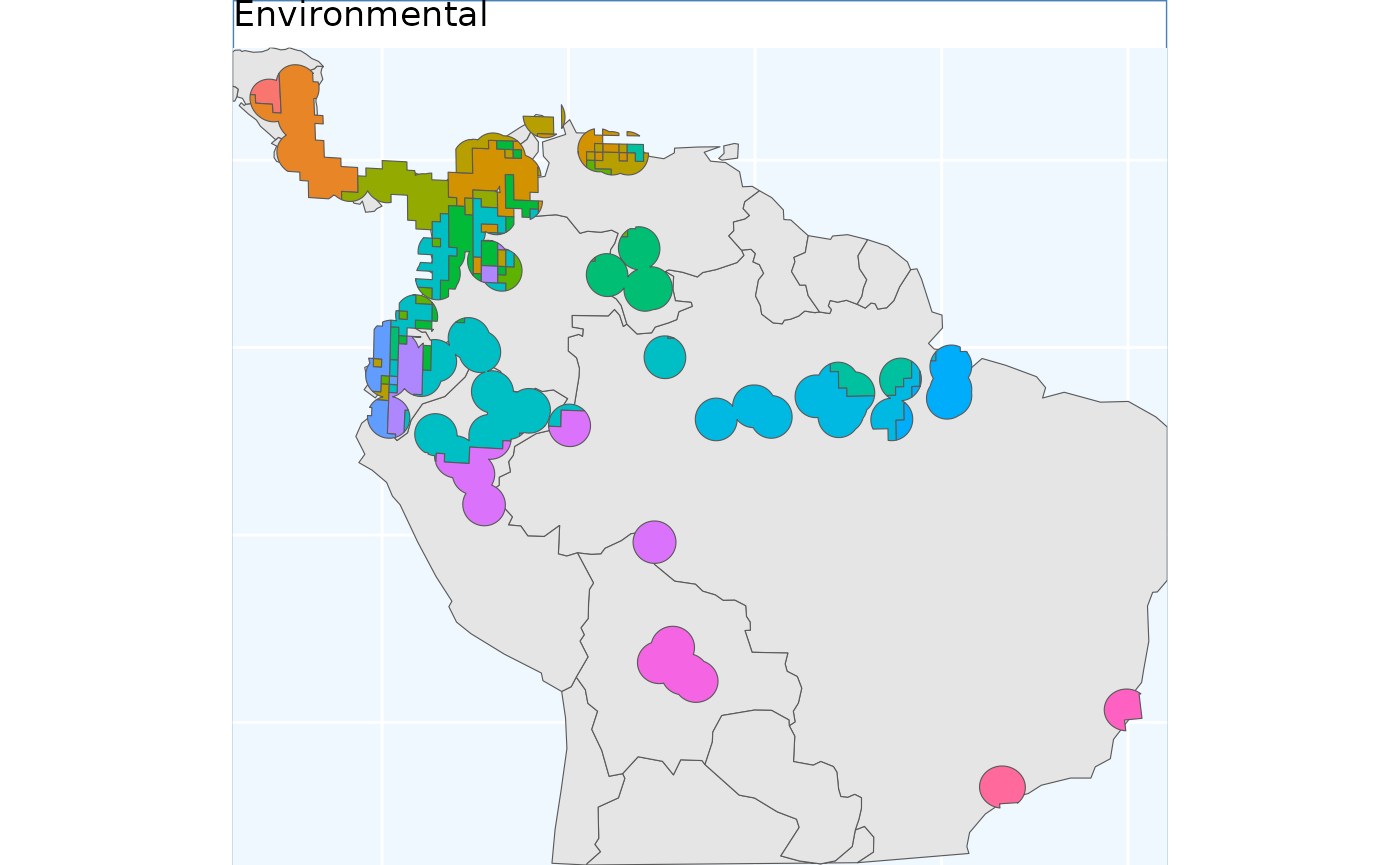

The function EnvironmentalBasedSample can take any of the three binary rasters created by PostProcessSDM as arguments for the template. Here we showcase the different results from using each of them.

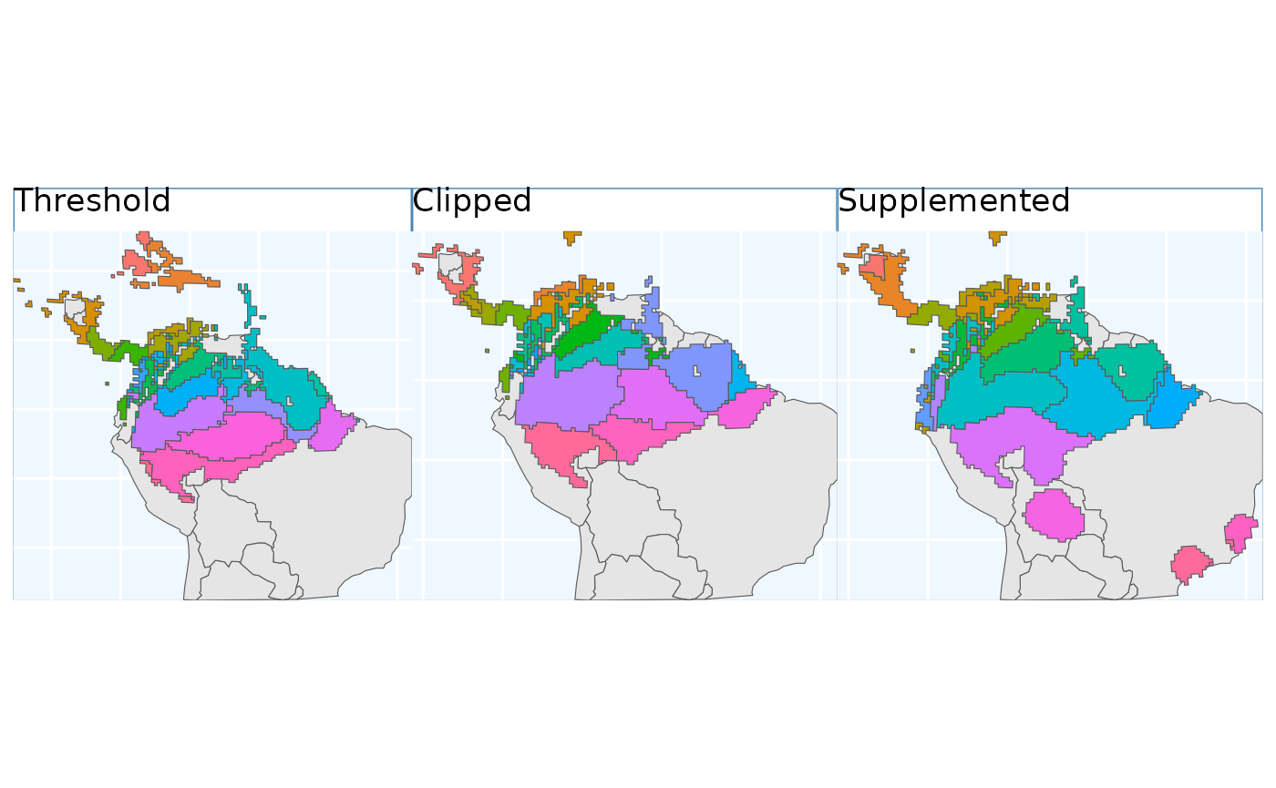
These plots can showcase the differences in results depending on which of the three input rasters are used. As with all sampling schemes, results vary widely depending on the spatial extent to which the functions are applied. Using the SDM output that has undergone thresholding results in the largest classified area. At first glance, the results may seem very different, but in Central America, they are largely consistent because it is near the Andes; large differences do exist in the Amazon Basin, but even there, some alignment between the systems is evident. Accordingly, the surface used for a species should match some evaluation criterion.

Using the threshold raster surface is a very good option if we do not want to ‘miss’ too many areas, whereas the clipped and supplemented options may be better suited for scenarios where we do not want to draw up clusters that lack any populations that can be collected from.

Comparision of different sampling schemes

So, we have some maps for you to look at! They all looked relatively similar to me when plotted one after another. Let’s plot them together and see if that’s still the case.

pbs.p + eas.p + os.p  +  ibdbs.p2 + ibr.p + ENVIbs.p + 
  plot_layout(ncol = 3)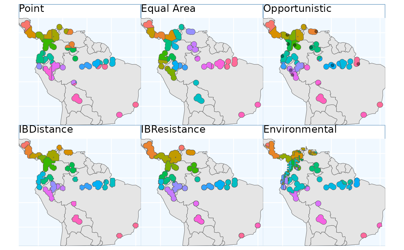

The geographic-based samples (here, Point, Equal Area, Opportunistic, and IBE) are quite similar. In my mind, isolation by distance (IBD) shows the biggest difference; it makes the most sense by splitting sampling areas along naturally occurring patches of the species range.

The application of PolygonBasedSample to the data is difficult to evaluate in the same way as the other data sets, but it did identify the desired sampling regions. We do not show it in this pane. Isolation by Resistance is similar to IBD; however, it makes fewer splits in Central America and instead picks them up in Peru.

Relative to IBR, Isolation by Environment tends to split locations across the Andes and the NW coastal regions of South America. The ranges are relatively contiguous enough to sensibly sample from. Contiguity of ranges in this approach can be controlled with the coord_wt argument.