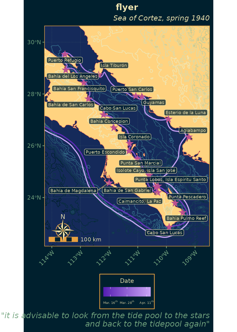
A dark-mode map • flyer

Introduction

The ExploreDataSets vignette builds a static map with a light “nautical” theme. Here we redo that map in a dark mode, borrowing the palette from the package’s hex sticker: a navy night sky, warm orange land, a purple route, and star markers for the collection stops.

library(flyer)
library(sf)
library(dplyr)
library(ggplot2)
library(ggrepel)
library(ggspatial)

The palette

The colors are picked to match the sticker. Anything you want to swap — say, the accent color for the route — just override the corresponding entry.

sticker_pal <- list(
  night        = '#00202e',  # deep navy background
  ocean        = '#152A5A',  # slightly lighter than night, for the plot panel 
  ocean_hi     = '#37718E',  # bathymetry hi end
  gold         = '#E8A040',  # hex border / land primary
  land_light   = '#ffd380',  # land fill (lighter orange)
  coral        = '#E86A55',  # land border / warm accent
  cream        = '#F0E5B0',  # ship body / label text
  mint         = '#74A57F',  # mast / topography
  purple       = '#531CB3',  # route (dark end)
  lavender     = '#C9A5F5',  # route (light end) / late-in-trip
  star_gold    = '#F5D060',  # city stars
  star_pink    = '#bc5090'   # tertiary highlight
)

The dark theme

A near-drop-in replacement for the light theme_nautical from the other vignette: same structure, but every element is repainted from the sticker palette.

theme_nautical_night <- function() {
  theme(
    aspect.ratio = 4/3,
    text = element_text(family = "Optima", color = sticker_pal$cream),

    axis.title = element_text(colour = sticker_pal$cream),
    axis.text = element_text(colour = sticker_pal$mint, face = "italic"),
    axis.text.x = element_text(hjust = 1, angle = 45),
    axis.ticks = element_line(colour = sticker_pal$mint),

    plot.title = element_text(hjust = 0.5, color = sticker_pal$pink, face = 'bold'),
    plot.subtitle = element_text(hjust = 1, face = 'italic', color = sticker_pal$cream),
    plot.caption = element_text(color = sticker_pal$mint, face = 'italic', size = 12),
    plot.background = element_rect(fill = sticker_pal$night, color = NA),

    panel.background = element_rect(fill = sticker_pal$ocean, color = NA),
    panel.border = element_rect(colour = sticker_pal$gold, fill = NA, linewidth = 0.7),
    panel.grid.major = element_line(
      colour = alpha(sticker_pal$mint, 0.3),
      linetype = 'dotted',
      linewidth = 0.25
    ),
    panel.grid.minor = element_blank(),

    legend.background = element_rect(fill = sticker_pal$night, color = sticker_pal$gold),
    legend.key = element_rect(fill = sticker_pal$night, color = NA),
    legend.text = element_text(size = 5, color = sticker_pal$cream),
    legend.title = element_text(size = 9, hjust = 0.5, color = sticker_pal$cream),
    legend.title.position = 'top',
    legend.key.size = unit(1, "line"),
    legend.position = "bottom",
    legend.spacing = unit(0.1, "line")
  )
}

Preparing the data

Same route/places join used in the light-mode vignette, plus a bounding box focused on the Sea of Cortez.

route <- left_join(
  route,
  st_drop_geometry(places),
  by = c('destination' = 'location_english')
) |>
  relocate(geometry, .after = last_col())

bb <- st_bbox(
  c(xmin = -114, xmax = -108.75, ymin = 22.5, ymax = 30.25),
  crs = st_crs(4326)
)

places <- st_crop(places, bb)

date_scale <- as.Date(
  quantile(
    as.numeric(route$date_arrive), na.rm = TRUE, probs = c(0.1, 0.5, 0.9)
    )
  )
date_lbls <- c(
  expression(paste("Mar. ", 16^th)),
  expression(paste("Mar. ", 28^th)),
  expression(paste("Apr. ", 11^th))
)

The map

Layered from the bottom up: bathymetry contours in cool blues, land in warm oranges (gold border on a lighter fill), topography contours in mint, the route as a purple gradient by arrival date, and the places as gold star-glyphs with cream labels on a dark backing.

ggplot() +

  # bathymetry from deep ocean to shallower shelves
  geom_sf(
    data = bathymetry,
    aes(color = elevation),
    lwd = 0.35
  ) +
  scale_color_gradient(
    'Depth (m)',
    low = sticker_pal$night,
    high = sticker_pal$ocean_hi,
    guide = 'none'
  ) +

  # land -- warm orange fill with a coral border
  geom_sf(
    data = land,
    fill = sticker_pal$land_light,
    color = sticker_pal$coral,
    linewidth = 0.25
  ) +

  # topography -- mint to cream gradient by elevation
  ggnewscale::new_scale_color() +
  geom_sf(
    data = topography,
    aes(color = elevation),
    linewidth = 0.45
  ) +
  scale_color_gradient(
    'Elevation (m)',
    low = sticker_pal$cream,
    high = alpha(sticker_pal$mint, 0.55),
    guide = 'none'
  ) +

  # route -- purple gradient along arrival date
  ggnewscale::new_scale_color() +
  geom_sf(
    data = route,
    aes(color = date_arrive),
    linewidth = 0.8
  ) +
  scale_color_gradient(
    'Date',
    low = sticker_pal$purple,
    high = sticker_pal$lavender,
    breaks = date_scale,
    labels = date_lbls
  ) +

  # places -- rendered as star glyphs
  geom_sf_text(
    data = places,
    label = '★',   # unicode filled star
    color = sticker_pal$star_pink,
    size = 6
  ) +
  ggrepel::geom_label_repel(
    data = places,
    aes(label = location_espanol, geometry = geometry),
    stat = 'sf_coordinates',
    size = 2.4,
    color = sticker_pal$cream,
    fill = alpha(sticker_pal$night, 0.75),
    label.size = NA,
    label.padding = 0.15,
    segment.color = alpha(sticker_pal$star_gold, 0.6)
  ) +

  # ambiance
  coord_sf(xlim = c(bb[1], bb[3]), ylim = c(bb[2], bb[4]), crs = 4326) +
  annotation_scale(
    bar_cols = c(sticker_pal$gold, sticker_pal$night),
    text_col = sticker_pal$cream,
    line_col = sticker_pal$gold
  ) +
  annotation_north_arrow(
    which_north = 'true',
    style = north_arrow_nautical(
      fill = c(sticker_pal$cream, sticker_pal$night),
      line_col = sticker_pal$gold,
      text_col = sticker_pal$cream
    )
  ) +
  theme_nautical_night() +
  labs(
    x = NULL, y = NULL,
    title = 'flyer',
    subtitle = 'Sea of Cortez, spring 1940',
    caption = '"it is advisable to look from the tide pool to the stars\nand back to the tidepool again"'
  )

Every color that drives the map lives in the sticker_pal list at the top of this vignette. Swapping a hex value there (say, brightening land_light or shifting purple toward blue) re-tints the entire figure without touching the geom code.