Introduction
The previous tutorials focus on the individual functions in the package but do little to show how to integrate them into common workflows for developing spatial products for sampling. Here we show a minimal example of how a curator may load occurrence data for a species, apply a couple of sampling approaches to these data, and save the results for use. We use two species native to the Southwestern United States and Mexico for this example. Eventually, we narrow our focus to just one species for brevity.
While we only have two species in the example, the code is set up to accommodate as many species as an analyst desires to process simultaneously. ## Data prep
You will need to install rgbif to follow along with this
example. rgbif is an amazing package maintained by ROpenSci
that provides access to the Global Biodiversity Information Facility
database from within R. Note that a (free and easy to get) GBIF profile
is required for larger data downloads, but for this example, all you
need is the R package.
library(safeHavens)
library(sf) # spatial data
library(rgbif) # species occurrence data.
library(spData) # example cartography data
library(dplyr) # general data handling
library(tidyr) # general data handling
library(purrr) # sub for lapplying functions across lists
library(ggplot2) ## for maps
Using rgbif, we’ll download occurrence data for a couple
of species, you can readily swap these out and supply a much longer list
of species use their proper GBIF codes.
This way, we can set up the code for mapping multiple species in a realistic manner.
## small subset of useful columns for example
cols = c('decimalLatitude', 'decimalLongitude', 'dateIdentified', 'species',
  'acceptedScientificName', 'datasetName', 'coordinateUncertaintyInMeters',
  'basisOfRecord', 'institutionCode', 'catalogNumber')

## download species data using scientificName, can use keys and lookup tables for automating many taxa.
cymu <- rgbif::occ_search(scientificName = "Vesper multinervatus", limit = 1000)

### check to see what CRS are in here, these days usually standardized to wgs84 (epsg:4326)
table( cymu[['data']]['geodeticDatum'])
geodeticDatum
WGS84
  737

## subset the data to relevant columns
cymu_cols <- cymu[['data']][,cols]

## repeat this again so a second set of data are on hand
bowa <- rgbif::occ_search(scientificName = "Bouteloua warnockii", limit = 1000)
bowa_cols <- bowa[['data']][,cols]

## contrived multispecies example.
spp <- bind_rows(bowa_cols, cymu_cols) |>
  drop_na(decimalLatitude, decimalLongitude) |> # any missing coords need dropped.
  st_as_sf(coords = c( 'decimalLongitude', 'decimalLatitude'), crs = 4326, remove = F)
We will make a very quick and simple basemap for use in the vignette
western_states <- spData::us_states |> ## for making a quick basemap.
  dplyr::filter(
    REGION == 'West' & ! NAME %in% ## SW / South focus rm, Northern states
      c('Montana', 'Washington', 'Idaho', 'Oregon', 'Wyoming')
    | ## OR -  to keep some of the steppe
   NAME %in% c('Oklahoma', 'Texas', 'Kansas')) |>
  dplyr::select(NAME, geometry) |>
  st_transform(4326)

ggplot() +
  geom_sf(data = western_states) +
  geom_sf(data = spp, aes(color = species, shape = species)) +
  theme_void() +
  theme(legend.position = 'bottom')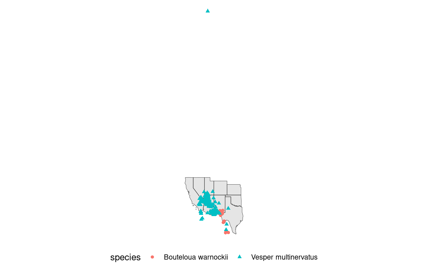
Quickly check the data for obvious errors. One point’s location is incorrect; its latitude is clearly wrong - we removed it below.
## check the outlying record.
arrange(spp, by = decimalLatitude, desc=TRUE) |>
  head(5) |>
knitr::kable()| decimalLatitude | decimalLongitude | dateIdentified | species | acceptedScientificName | datasetName | coordinateUncertaintyInMeters | basisOfRecord | institutionCode | catalogNumber | geometry |
|---|---|---|---|---|---|---|---|---|---|---|
| 26.24360 | -102.8460 | NA | Bouteloua warnockii | Bouteloua warnockii Gould & Kapadia | NMNH Extant Biology | NA | PRESERVED_SPECIMEN | US | US 3419592 | POINT (-102.846 26.2436) |
| 26.24361 | -102.8461 | NA | Bouteloua warnockii | Bouteloua warnockii Gould & Kapadia | Estudio biosistemático del género Bouteloua de México | 50 | PRESERVED_SPECIMEN | CIIDIR-IPN | 13158 | POINT (-102.8461 26.24361) |
| 26.24361 | -102.8461 | NA | Bouteloua warnockii | Bouteloua warnockii Gould & Kapadia | Computarización de colecciones y adquisición de infraestructura (mobiliario) para el herbario CIIDIR-Durango | NA | PRESERVED_SPECIMEN | CIIDIR-IPN | 34657 | POINT (-102.8461 26.24361) |
| 26.30530 | -101.3430 | NA | Bouteloua warnockii | Bouteloua warnockii Gould & Kapadia | NMNH Extant Biology | NA | PRESERVED_SPECIMEN | US | US 3481177 | POINT (-101.343 26.3053) |
| 26.30833 | -101.3583 | NA | Bouteloua warnockii | Bouteloua warnockii Gould & Kapadia | Estudio biosistemático del género Bouteloua de México | 50 | PRESERVED_SPECIMEN | UAAAN | 18673 | POINT (-101.3583 26.30833) |
## remove the mis-geocoded record based on its latitude.
spp <- filter(spp, decimalLatitude <= 40)
A few tools exist for quickly cleaning GBIF data we will not get into them here. However, tey should make cleaning and subsetting records much easier for users. gatoRs is a recent package and great choice.
Below we map the data again, - accounting for the removal of the mis-geocoded point, and keep the ggplot around as a basemap for the rest of the vignette.
bb <- st_transform(spp, 5070) |>
  st_buffer(100000) |>
  st_transform(4326) |>
  st_bbox()

western_states <- st_crop(western_states, bb)

base <- ggplot() +
  geom_sf(data = western_states, color = 'white') +
  geom_sf(data = spp, aes(color = species)) +
  theme_void() +
  theme(legend.position = 'bottom') +
  guides(color = guide_legend(nrow = 2))

base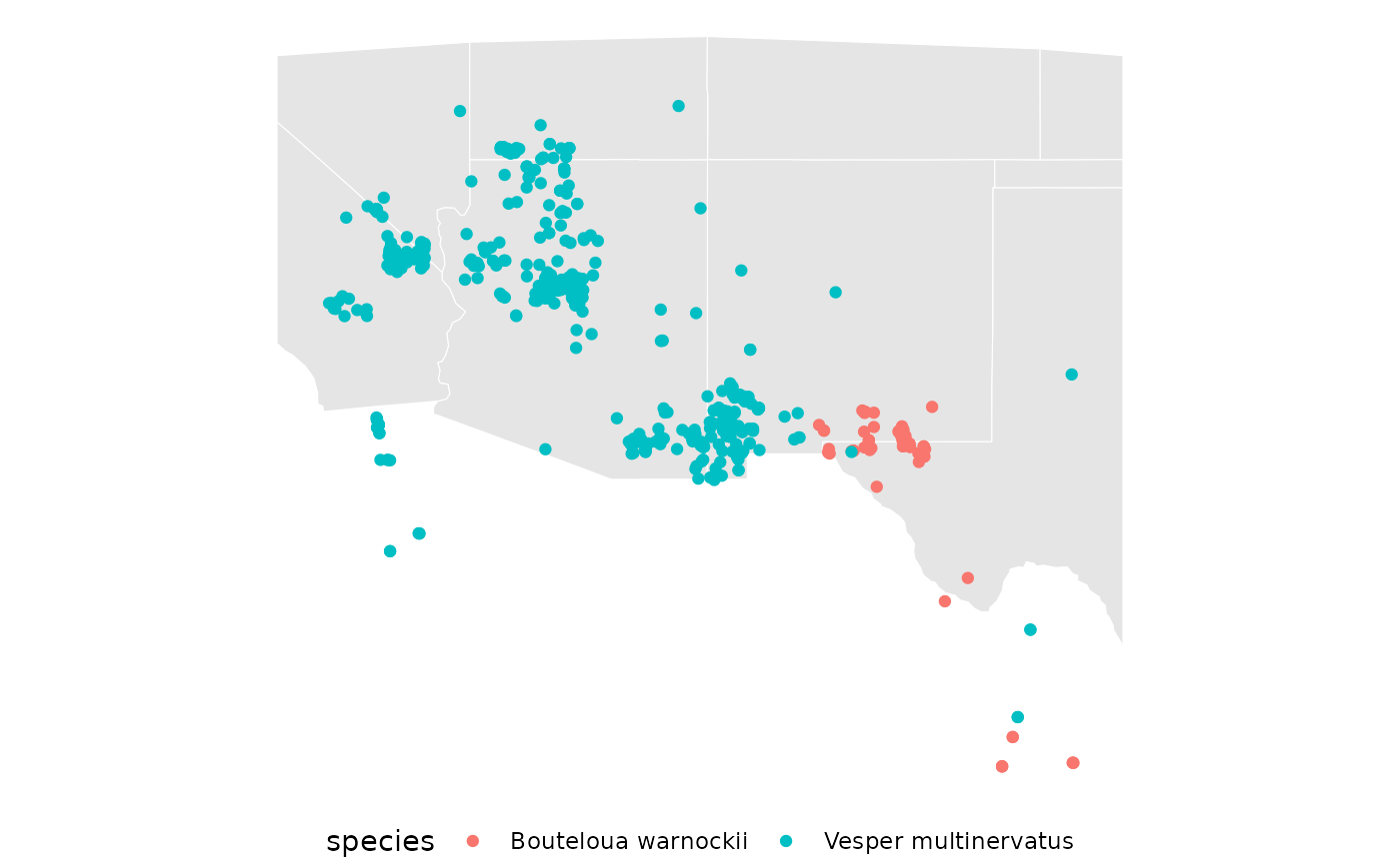
using safeHavens
Now we will use the safeHavens functionality in our setup environment with GBIF data.
Create species ranges
We will showcase two methods for generating species-range geometries,
which are used by most of the packages’ functions. Both of these rely on
the st_concave_hull function from sf.
st_concave_hull has a ratio parameter that controls the
elasticity of the hull; ratio = 1 creates a convex hull (akin to the
st_convex_hull function, also in sf), and ratio = 0.0
creates a true concave hull. Results below a ratio of 0.4 appear too
narrow for both of these species.
sppL <- split(spp, f = spp$species)

concavities <- function(x, d, rat){

  species <- x[['species']][1]
  out <- st_transform(x, 5070) |>
    st_buffer(dist = d) |>
    st_union() |>
    st_concave_hull(ratio = rat) |>
    st_sf() |>
    rename(geometry = 1) |>
    mutate(species, .before = geometry)

}

spp_concave <- sppL |>
  purrr::map(~ concavities(.x, d = 20000, rat = 0.4))
spp_convex <- sppL |>
  purrr::map(~ concavities(.x, d = 20000, rat = 1.0))

rm(concavities)
Visualize the concave hulls.
base +
  geom_sf(data = spp_concave[[1]], aes(fill = species), alpha = 0.2) +
geom_sf(data = spp_concave[[2]], aes(fill = species), alpha = 0.2) 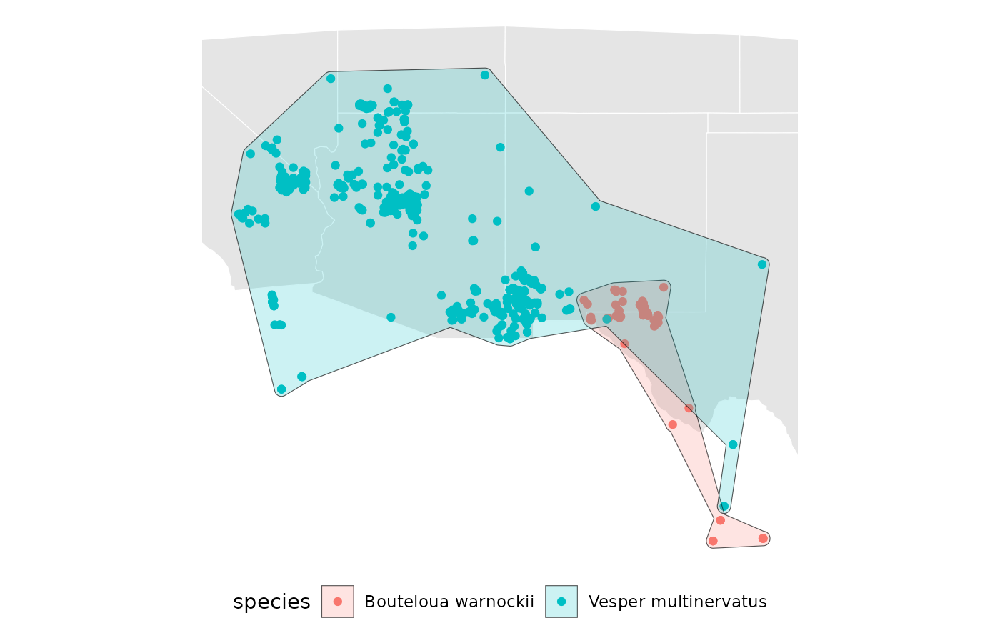
Visualize the convex hulls.
base +
  geom_sf(data = spp_convex[[1]],  aes(fill = species), alpha = 0.2) +
geom_sf(data = spp_convex[[2]], aes(fill = species), alpha = 0.2) 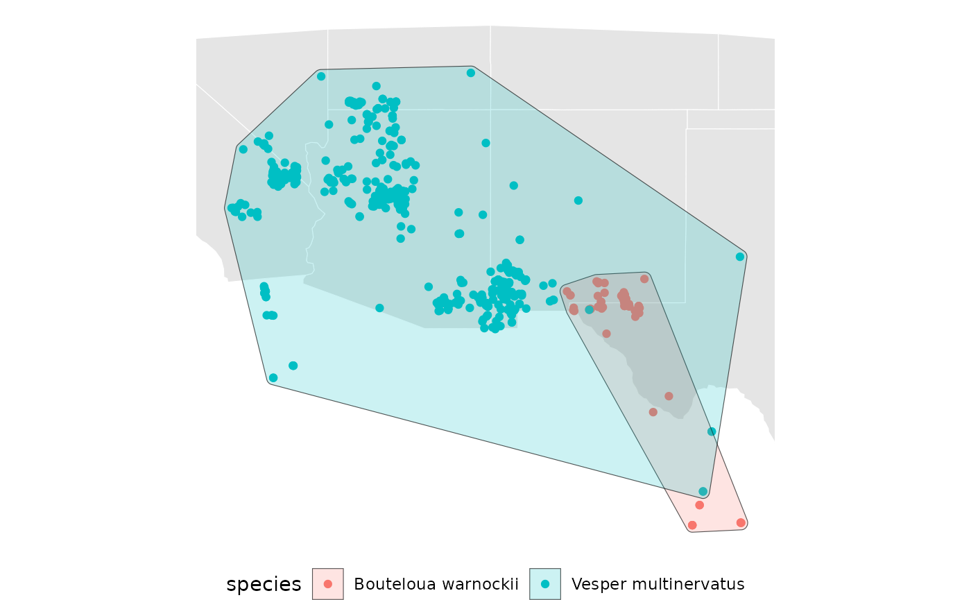
For the sake of the example, we will use only the concave ranges with a ratio of 0.4 going forward.
Perform sampling for the species ranges
First, we will perform equal area sampling with a relatively small number of points and repetitions.
eas <- spp_concave |>
  purrr::map(~ EqualAreaSample(.x, n = 10, pts = 250, planar_proj = 5070, reps = 25))

base +
  geom_sf(
    data = eas[[2]][['Geometry']],
    aes(fill = factor(ID)),
    alpha = 0.2
    ) +
labs(fill = 'region') 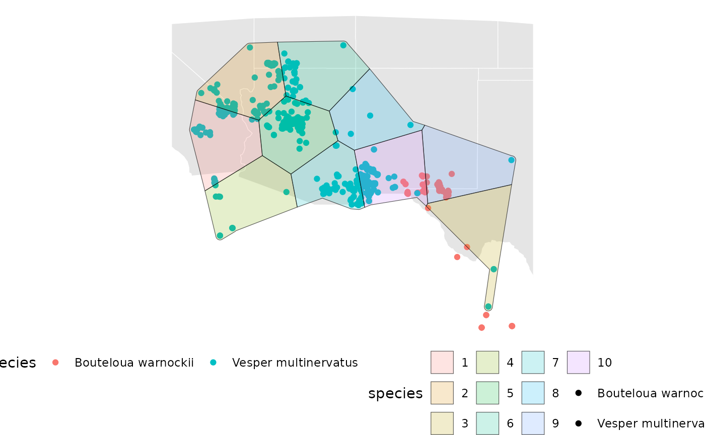
The plot above shows only the results for Vesper multinervatus.
Below, we perform isolation-by-distance (IBD)- based sampling. It is called within a purr::map(~), operating on the spp_concave object. This could be swapped out for other safeHavens functions.
# create an arbitrary template for example - best to do this over your real range of all species collections
# so that it can be recycled across species.
template <- terra::rast(
  terra::ext(bb), crs = terra::crs(spp), resolution = c(0.1, 0.1)
  )
terra::values(template) <- 0

# the species range now gets 'burned' into the raster template.
spp_concave <- purrr::map(spp_concave, \(x) {
  st_as_sf(x) |>
    mutate(Range = 1, .before = geometry) |>
    st_transform(4326) |>
    terra::rasterize(template, field = 'Range')
})

## the actual sampling happens here within `map`
ibd_samples <- spp_concave |>
  purrr::map(~ IBDBasedSample(.x, n = 10, fixedClusters = FALSE, template = template, planar_proj = 5070))

base + ## visualize for a single taxon.
  geom_sf(
    data = ibd_samples[[1]][['Geometry']],
    aes(fill = factor(ID)),
    alpha = 0.2
    )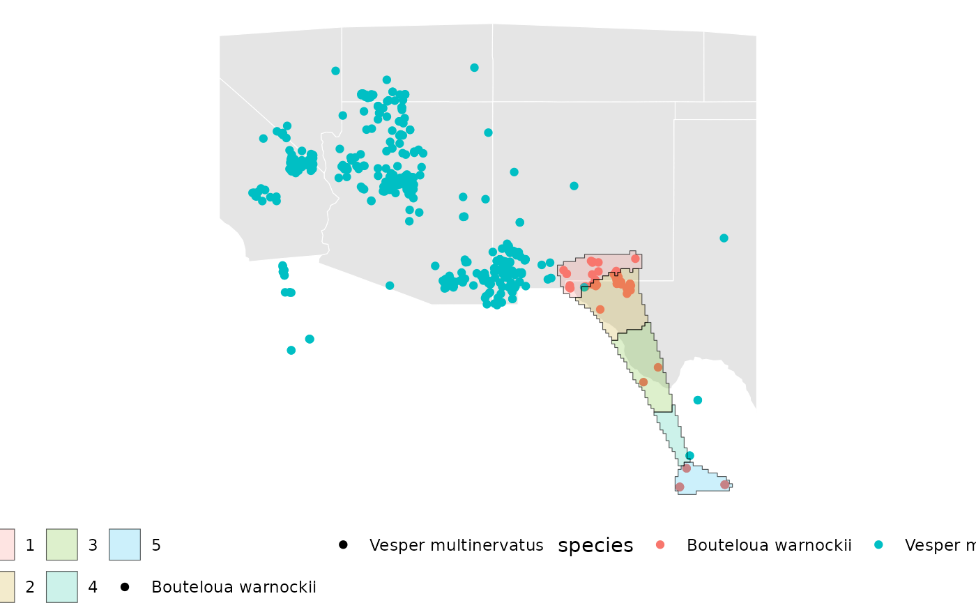
The isolation-by-distance plot above highlights individual sample areas for Bouteloua warnockii.
prioritize sample areas
In addition to creating spatial geometries to guide sampling efforts,
safeHavens can also provide visual guidance on general
areas where germplasm can be sampled to maximise the distance between
samples. Please note that while safeHavens can offer
suggestions of where to sample, and where should be prioritised, these
suggestions may not align with reality - so consider these rules of
thumb! I have made a couple of hundred large native seed collections and
coordinated a couple hundred more, for many years, and I argue that
beggars cannot be choosers. Hence, basing deliverable metrics purely
around data like this can be difficult - some degree of reporting
autonomy must be maintained.
The function PrioritizeSample offers two levels of
prioritisation. The coarser level will suggest a relative order for the
sample areas to be sampled, from 1:n; the function seeks to minimise the
variance (a related measure) between samples as more are collected. In
effect, it tries to stratify the sampling across the species range. The
second part of the function is almost a ‘heatmap’ which can be used to
show concentric rings around the geographic centre of each sample unit.
Keeping the number of rings low allows for some pragmatic communication
of more desirable/less desirable portions of the range to ideally
collect in.
ibd_samples_priority <- ibd_samples |>
  purrr::map(~ st_transform(.x$Geometry, 5070)) |>
  purrr::map(~ list(PrioritizeSample(.x, n_breaks = 3)))

base +
  geom_sf(
    data = ibd_samples_priority[[2]][[1]][['Geometry']],
    aes(fill = factor(Level)),
    alpha = 0.2
    ) +
labs(fill = 'Priority Level') 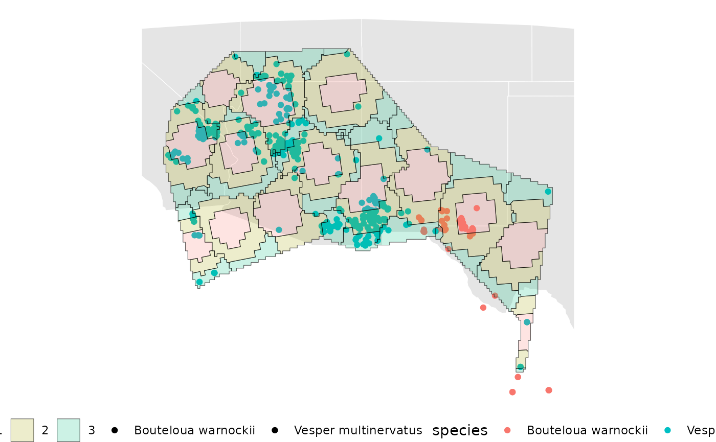
The map above shows a possible general order to guide the prioritisation of individual sample areas, along with simplified visuals of where within those areas to target.
wrapping up
Upon completion of using safeHavens, results should be written to individual geopackages for long-term storage. A significant benefit of a geopackage is its ability to store multiple geometry types (polygons, points, rasters, etc.), which can be lost when stored in separate directories.
Here is how to write out species data.
## create a directory to hold the outputs
p2Collections <- file.path('~', 'Documents', 'WorkedExample_Output')
dir.create(p2Collections, showWarnings = FALSE)

## we will only save the template raster once since it is recycled across taxa.
dir.create(
  file.path(p2Collections, 'IBD_raster_template'),
  showWarnings = FALSE
  )

terra::writeRaster(template,
  filename = file.path(
    p2Collections, 'IBD_raster_template', 'IBD_template.tif'),
    overwrite = FALSE)

## save each species as a unique geopackage.
## geopackage will keep contents from getting split up.
for(i in seq_along(sppL)){

  fp = file.path(
    p2Collections,
    paste0(gsub(' ', '_', sppL[[i]]$species[1]), '.gpkg')
    )

  ### GBIF occurrence points
  st_write(
    sppL[[i]],
    dsn = fp,
    layer = 'occurrence_points',
    quiet = TRUE
    )

  ### results of equal area sampling
  st_write(
    eas[[i]]$Geometry,
    dsn = fp,
    layer =  'equal_area_samples',
    quiet = TRUE,
    append = TRUE
    )

  ### ibd based sample (can be reconstructed from the hulls of ibd samples priority)
  st_write(
    ibd_samples[[i]]$Geometry,
    dsn = fp,
    layer =  'ibd_samples',
    quiet = TRUE,
    append = TRUE
    )

  ### prioritized information for the IBD samples.
  st_write(
    ibd_samples_priority[[i]][[1]]$Geometry,
    dsn = fp,
    layer =  'ibd_sampling_priority',
    quiet = TRUE,
    append = TRUE
    )

 ## print object size of saved data.
  message(
    format(
      object.size(fp),
      standard = "IEC",
      units = "MiB",
      digits = 4)
      )
}