Species Distribution Modelling

Background

This vignette details the steps required to create a Species Distribution Model (SDM) using the functions provided in safeHavens. The SDM is required to use the EnvironmentalBasedSample function, which is the most complex sampling scheme provided in the package. The SDM is created using an elastic net generalized linear model implemented via the glmnet package. The SDM is then post-processed to create a binary raster map of suitable and unsuitable habitat, that is used to rescale the environmental predictor variables according to their contributions to the model. These rescaled variables are then used in a clustering algorithm to partition the species range into environmentally distinct regions for germplasm sampling.

The goal of most SDM’s is to create a model that accurately predicts where a species will be located in environmental space and can then be predicted in geographic space. The goal of these models is to understand the degree and direction to which various environmental features correlate with a species observed range. This model is not intended to replace a well-structured and thought-out SDM; rather, it is intended to provide a quick model that can be used to inform sampling strategies.

About

While the authors are prone to creating many ‘advanced’ SDMs models and in-house pipelines for developing them, we think that the juice is not worth the squeeze and rely on a few powerhouse R packages to do the heavy lifting. The main packages used are dismo, caret, glmnet, CAST, and terra. The dismo package provides a user-friendly interface for working with species occurrence and raster data, as well as some helper functions for thresholding and evaluating models. The caret package provides a nice interface for working with machine learning models, and the glmnet package provides the elastic net model. The CAST package provides functions for spatially informed cross-validation, which is important for SDMs. The terra package provides functions for working with raster data. All of these packages are well documented, and maintained.

Steps to create an SDM

prep data

library(safeHavens)

First you will need georeference occurrence data for your species of interest. For common species we recommened the rgbif package to download occurrence data from GBIF.

Here to maintain a smaller package size, and integrate with the tutorial in dismo we use a built in data set for Bradypus variegatus (Brown-throated sloth). We do this to also leverage the raster data provided in dismo as well.

x <- read.csv(file.path(system.file(package="dismo"), 'ex', 'bradypus.csv'))
x <- x[,c('lon', 'lat')]
x <- sf::st_as_sf(x, coords = c('lon', 'lat'), crs = 4326)

planar_proj <- 3857 # Web Mercator for planar distance calcs

files <- list.files(
  path = file.path(system.file(package="dismo"), 'ex'), 
  pattern = 'grd',  full.names=TRUE )
predictors <- terra::rast(files) # import the independent variables

fit the model

Here we fit as SDM using elasticSDM. For arguments it requires occurrence data x, a raster stack of predictors, a quantile_v that is an offset used to create pseudo-absence data, and a planar_proj used to calculate distances between occurrence data and possible pseudo-absence points. The quantile_v is used to create pseudo-absence data by calculating the distance from each occurrence point to the nearest neighbor, and then selecting a quantile of these distances to create a buffer around each occurrence point. Points outside of this buffer are used pseudo-absences.

sdModel <- elasticSDM(
  x = x,
  predictors = predictors,
  quantile_v = 0.025,
  planar_proj = planar_proj
  )
Warning: 
Grid searches over lambda (nugget and sill variances) with  minima at the endpoints: 
  (GCV) Generalized Cross-Validation 
   minimum at  right endpoint  lambda  =  1.656291e-07 (eff. df= 174.8 )
Warning: 
Grid searches over lambda (nugget and sill variances) with  minima at the endpoints: 
  (GCV) Generalized Cross-Validation 
   minimum at  right endpoint  lambda  =  1.656291e-07 (eff. df= 174.8 )
Warning: 
Grid searches over lambda (nugget and sill variances) with  minima at the endpoints: 
  (GCV) Generalized Cross-Validation 
   minimum at  right endpoint  lambda  =  1.656291e-07 (eff. df= 174.8 )

Under the hood this function uses caret to help out with glmnet, as it provides output which is very easy to explore and interact with. Elastic net modelS bridge the world of lasso and ridge regression by blending the alpha parameter. Lasso has an alpha of 0, while Ridge has an alpha of 1. Lasso regression will perform automated variable selection, and can drop (or ‘shrink’) features from a model, whereas Ridge will keep all variables and if correlated features exist split contributions between them. An elastic net blends this propensity to drop or retain variables whenever it is used. caret will test a range of alphas to determine how much ridge or lasso regression characteristics are best for the data at hand.

MAKE A NOTE ABOUT THE PCNM MORAN EIGNENVECTORS HERE TOO.

explore the output

{r Explore SDM output - Different alpha}sdModel$CVStructure coef(sdModel$Model, s = "lambda.min")

Here we can see how the elastic net decided that is the top model. We used Accuracy rather than Kappa as the main criterion for model selection.

sdModel$ConfusionMatrix
Confusion Matrix and Statistics

          Reference
Prediction  0  1
         0 16  1
         1  7 21
                                        
               Accuracy : 0.8222        
                 95% CI : (0.6795, 0.92)
    No Information Rate : 0.5111        
    P-Value [Acc > NIR] : 1.465e-05     
                                        
                  Kappa : 0.6464        
                                        
 Mcnemar's Test P-Value : 0.0771        
                                        
            Sensitivity : 0.9545        
            Specificity : 0.6957        
         Pos Pred Value : 0.7500        
         Neg Pred Value : 0.9412        
             Prevalence : 0.4889        
         Detection Rate : 0.4667        
   Detection Prevalence : 0.6222        
      Balanced Accuracy : 0.8251        
                                        
       'Positive' Class : 1

Here we can see how our selected model works on predicting the state of test data. Note these accuracy results are slightly higher than those from the CV folds. This is not a bug, CV folds are testing on their own holdouts, while this is a brand new set of holdouts. The main reason the confusion matrix results are likely to be higher is due to spatial auto-correlation which are not address in a typical ‘random split’ of test and train data. In order to minimize the effects of spatial-autocorrelation on our model we use CAST under the hood which allows for spatially informed cross validation.

Consider the output from CVStructure to be a bit more realistic.

binarize the output

terra::plot(sdModel$RasterPredictions)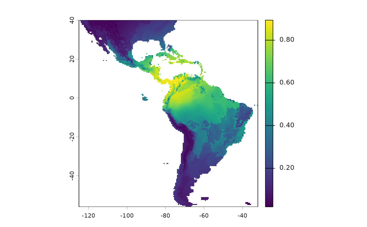

SDM’s produce continuous surfaces displaying the predicted probability of suitable habitat across a landscape. However binary surfaes (Yes/No Suitable), i.e. is it more or less probable that suitable habitat for this taxon exists in this particular location (grid cell)? are often required from them; the function PostProcessSDM is used to binarize the predictions.

Going from a continuous surface to a binary surface loses information. The goal of the binary surface is to understand where the species is likely to be found, and then sample germplasm from these areas. There are many ways to threshold a SDM, and many caveats associated with this process; Frank Harrell has written on the topic of post-processing in statistics.

Historically, when assessing probability output 0.5 probability was used as a threshold, probabilities beneath it considered ‘Not Suitable / No’, while probabilities above are classified as ‘Suitable / Yes’. This works for some cases, but thresholding is outside the domain of statistics and in the realm of practice. My motto for implementing models, is a slight elaboration of George Box’s aphorism, “All models are wrong, some are useful - how do you want to be wrong?”. Our goal of sampling for germplasm conservation is to maximize the representation of allelic diversity across the range of a species. To achieve this, we need an understanding of the species actual range, hence it is better to predict the species present where it is not, than to predict it absent where it actually grows. Accordingly, my default thresholding statistic is Sensitivity. However, our function supports all threshold options in dismo::threshold.

You may be wondering why this function is named PostProcessSDM rather ThresholdSDM, the reason for this discontinuity is that the function performs additional processes after thresholding. Geographic buffers are created around the intitial occurence points to ensure that none of the known occurrence points are ‘missing’ from the output binary map. This is a two edged sword, where we are again address the notion of dispersal limitation, and realize that not all suitable habitat is occupied habitat.

What the PostProcessSDM function does is it again creates cross validation folds, and selects all of our training data. In each fold if then calculates the distance from each occurrence point to it’s nearest neighbor. We then summarize these distances and can understand the distribution of distances as a quantile. We use a selected quantile, to then serve as a buffer. Area with predicted suitable habitat outside of this buffer become ‘cut off’ (or masked) from the binary raster map, and areas within buffer distance from known occurrences which are currently masked are reassigned as probabilities. The theory behind this process in underdeveloped and nascent, it does come down to the gut of an analyst. With the Bradypus data set I use 0.25 as the quantile, which is saying “Neighbors are generally 100km apart, I am happy with the risk of saying that 25km within each occurrence is occupied suitable habitat”. Increasing this value to say 1.0 will mean that no suitable habitat is removed, decreasing it makes maps more conservative. The cost with increasing the distances greatly is that the sampling methods may then puts grids in many areas without populations to collect from.

threshold_rasts <- PostProcessSDM(
  rast_cont = sdModel$RasterPredictions, 
  test = sdModel$TestData,
  train = sdModel$TrainData,
  planar_proj = planar_proj,
  thresh_metric = 'sensitivity', 
  quant_amt = 0.5
  )
1000 prediction points are sampled from the modeldomain

We can compare the results of applying this function side by side using the output from the function.

terra::plot(threshold_rasts$FinalRasters)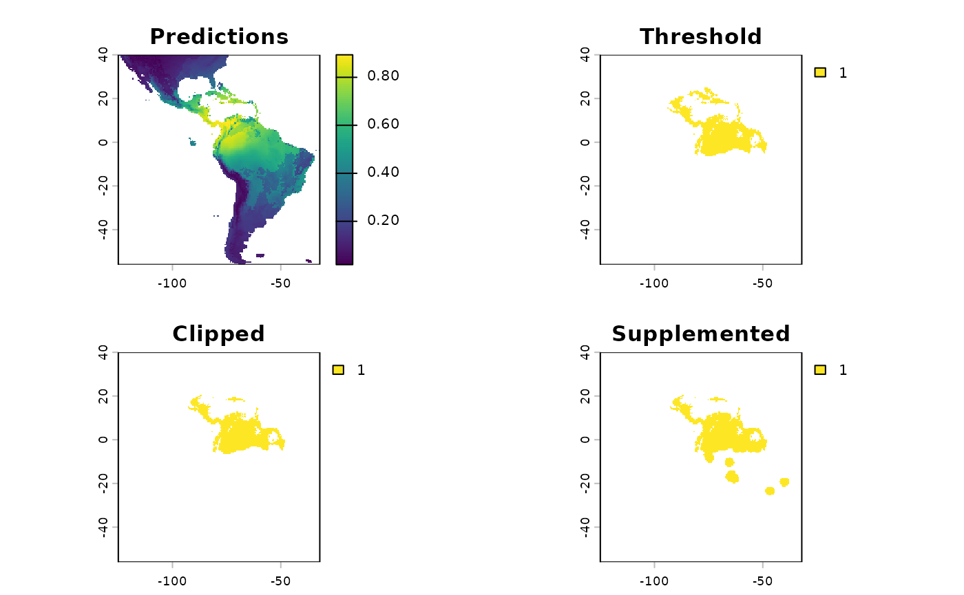

rescale predictor variables

glmnet is used for three main reasons, 1) it gives directional coefficients and documents how each 1 unit increase in an independent variable varies the response. 2) It maintains automated feature selection reducing the work an analyst needs to do. 3) glmnet re-scales all variables before model generation combined with beta-coefficients allows for partitioning environmental space into regions that are environmentally similar for the individual species.

In this way our raster stack becomes representative of our model, we can then use these values as the basis for hierarchical cluster later on.

Below we create a copy of the raster predictions where we have standardized each variable, so it is equivalent to the input to glmnet, and then mulitplied by its beta-coefficient. We will also write out these beta coefficients with the writeSDMresults function right afterwards.

rr <- RescaleRasters(
  model = sdModel$Model,
  predictors = sdModel$Predictors, 
  training_data = sdModel$TrainData, 
  pred_mat = sdModel$PredictMatrix)

terra::plot(rr$RescaledPredictors)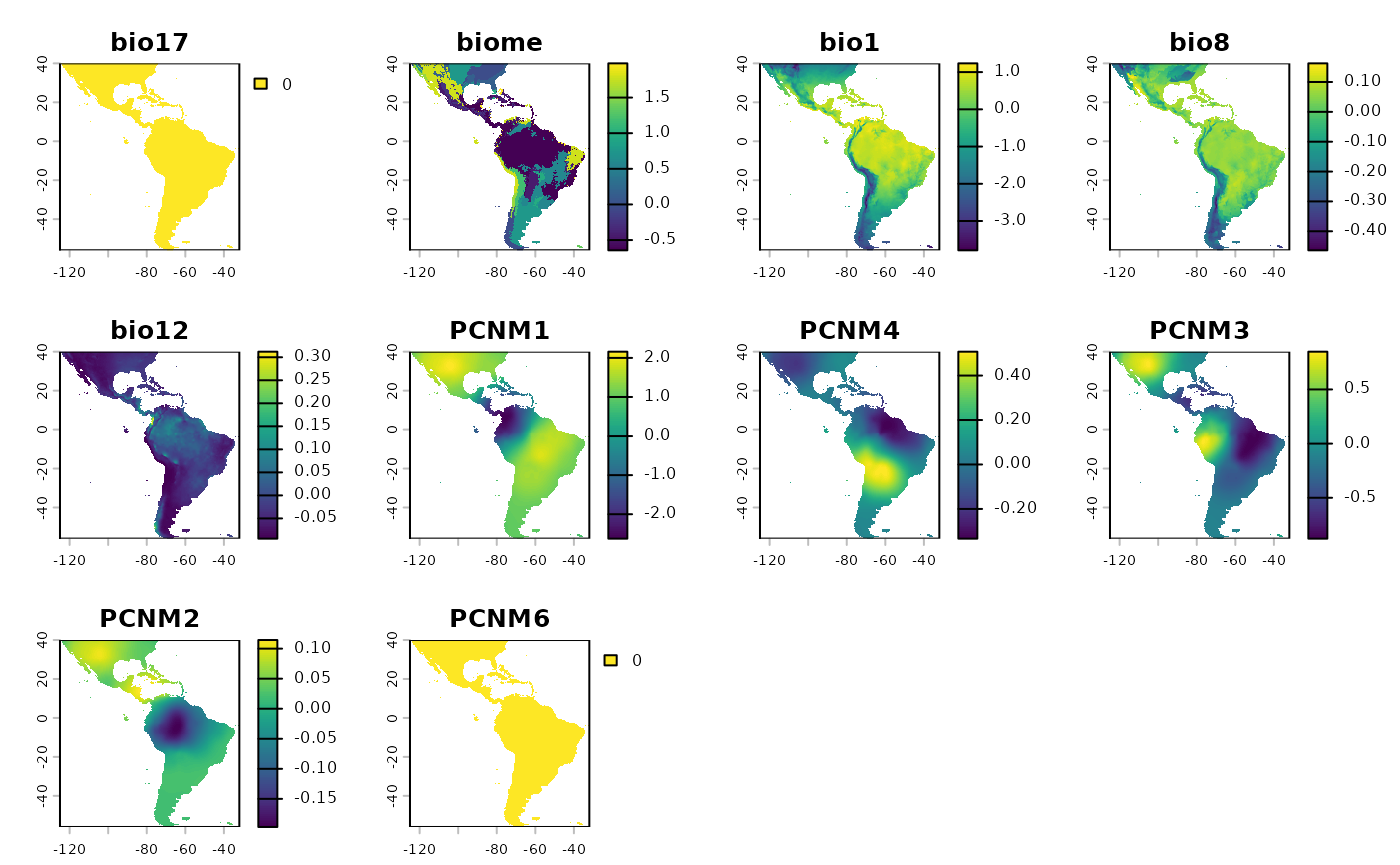

We can see that the variables are ‘close’ to being on the same scale, this will work in a clustering algorithm. If any of the layers are all the same color (maybe yellow?) that means they have no variance, that’s a term that was shrunk from the model. It will be dealt with internally in a future function. The scales of the variables are not exact, because they are weighed by their coefficients in the model

{r Show beta Coefficients from model print(rr$BetaCoefficients)

We can also look at the coefficients for each variable. glmnet returns the ‘untransformed’ variables, i.e. the coefficients on the same scale as the input rasters, we calculate the BC right afterwards.

safeHavens generates all kinds of things as it runs through the functions elasticSDM, PostProcessSDM, and RescaleRasters. Given that one of these sampling scheme may be followed for quite some time, it is best practice to save many of these objects.

save results

bp <- '~/Documents/assoRted/StrategizingGermplasmCollections'

writeSDMresults(
  cv_model = sdModel$CVStructure, 
  pcnm = sdModel$PCNM, 
  model = sdModel$Model, 
  cm = sdModel$ConfusionMatrix, 
  coef_tab = rr$BetaCoefficients, 
  f_rasts = threshold_rasts$FinalRasters,
  thresh = threshold_rasts$Threshold,
  file.path(bp, 'results', 'SDM'), 'Bradypus_test')

# we can see that the files were placed here using this. 
list.files( file.path(bp, 'results', 'SDM'), recursive = TRUE )

wrapping up

And there you have it, all the steps to make a species distribution model - or rather to get the coefficients from a species distribution model! We will play around with it as an example data set to compare our buffered distance results to at the end - head over to the next vignette!

Species Distribution Models