safeHavens includes one function for population-level
data.
prepare data
Load the required packages.
For this vignette, we will use the Bradypus data included in the
dismo package.
x <- read.csv(file.path(system.file(package="dismo"), 'ex', 'bradypus.csv'))
x <- x[,c('lon', 'lat')]
x <- sf::st_as_sf(x, coords = c('lon', 'lat'), crs = 4326)
We will now create the same base map used in the
GettingStarted example. While this chunk is ‘hidden’ in the
rendered man pages, it remains present in the raw vignette
documents.
Warning: attribute variables are assumed to be spatially constant throughout
all geometries
Unlike other functions in the package that use sf objects, this function instead uses a simple site data frame for more efficient calculations.
The KMedoidsBasedSample function requires a list as
input, consisting of two elements: (1) a distance matrix, and (2) a data
frame containing site locations and relevant attributes. Ensure both
elements are present when calling this function. The required columns in
the data frame are: site_id, coord_uncertainty, lon, and lat. Please
verify your data frame includes each of these columns to ensure proper
function performance.
n_sites <- nrow(x)
df <- data.frame(
  site_id = seq_len(n_sites),
  required = FALSE,
  coord_uncertainty = 0,
  lon = sf::st_coordinates(x)[,1],
  lat = sf::st_coordinates(x)[,2]
)

knitr::kable(head(df))| site_id | required | coord_uncertainty | lon | lat |
|---|---|---|---|---|
| 1 | FALSE | 0 | -65.4000 | -10.3833 |
| 2 | FALSE | 0 | -65.3833 | -10.3833 |
| 3 | FALSE | 0 | -65.1333 | -16.8000 |
| 4 | FALSE | 0 | -63.6667 | -17.4500 |
| 5 | FALSE | 0 | -63.8500 | -17.4000 |
| 6 | FALSE | 0 | -64.4167 | -16.0000 |
The distance matrix, which is the second required element of the
input list, can be generated using the greatCircleDistance
function from this package. Use this instead of
sf::st_distance to keep unit consistency, as the units
differ. If using sf::st_distance, always convert the units
to match those of greatCircleDistance to ensure correct
results. As an alternative, you can use an environmental distance matrix
derived from the first two axes of a PCA, as described in more detail
below.
dist_mat <- sapply(seq_len(nrow(df)), function(i) {
   greatCircleDistance(
     df$lat[i], df$lon[i],
     df$lat, df$lon
   )
 })
The optimisation routine requires at least one specified site. Here, we will select the site location closest to the geographic centre of all sites as the required site.
Normally, this refers to existing accessions, administrative units, or nature preserves that support the germplasm collection by already possessing samples or guaranteed access.
dists2c <- greatCircleDistance(
  median(df$lat),
  median(df$lon),
  df$lat,
  df$lon
)
df[order(dists2c)[1],'required'] <- TRUE
This function bootstraps sites to simulate the species’ true distribution and bootstraps coordinate uncertainty for each site. Here, we will randomly assign 20% of the sites to have coordinate uncertainty ranging from 1 km to 40 km. Coordinate uncertainty is always measured in meters.
Run KMedoidsBasedSample based only on geographic distances
The function takes two inputs: a distance matrix and site data.
test_data <- list(
  distances = dist_mat,
  sites = df
  )

str(test_data)
List of 2
 $ distances: num [1:116, 1:116] 0 1.83 714.09 807.71 797.93 ...
 $ sites    :'data.frame':  116 obs. of  5 variables:
  ..$ site_id          : int [1:116] 1 2 3 4 5 6 7 8 9 10 ...
  ..$ required         : logi [1:116] FALSE FALSE FALSE FALSE FALSE FALSE ...
  ..$ coord_uncertainty: num [1:116] 0 0 0 0 0 ...
  ..$ lon              : num [1:116] -65.4 -65.4 -65.1 -63.7 -63.9 ...
  ..$ lat              : num [1:116] -10.4 -10.4 -16.8 -17.4 -17.4 ...
The function KMedoidsBasedSample has several arguments
used to control run parameters.
st <- system.time( {
    geo_res <- KMedoidsBasedSample(
       ## reduce params from defaults
       ##  for a quick run.

      input_data = test_data,
      n = 5,
      n_bootstrap = 10,
      dropout_prob = 0.1,
      n_local_search_iter = 10,
      n_restarts = 2
    )
  }
)
Sites: 116 | Seeds: 1 | Requested: 5 | Coord. Uncertain: 19 | BS Replicates: 10
  |                                                                              |                                                                      |   0%  |                                                                              |=======                                                               |  10%  |                                                                              |==============                                                        |  20%  |                                                                              |=====================                                                 |  30%  |                                                                              |============================                                          |  40%  |                                                                              |===================================                                   |  50%  |                                                                              |==========================================                            |  60%  |                                                                              |=================================================                     |  70%  |                                                                              |========================================================              |  80%  |                                                                              |===============================================================       |  90%  |                                                                              |======================================================================| 100%
The function runs quickly with a few bootstrap or site samples, but it will take longer with more complex scenarios. We recommend using at least 999 bootstraps for real-world applications.
knitr::kable(st)| x | |
|---|---|
| user.self | 27.512 |
| sys.self | 0.049 |
| elapsed | 27.563 |
| user.child | 0.000 |
| sys.child | 0.000 |
return output structure
Five objects are returned by the function.
str(geo_res)
List of 5
 $ input_data     :'data.frame':    116 obs. of  10 variables:
  ..$ site_id          : int [1:116] 47 21 5 83 100 6 106 19 95 86 ...
  ..$ required         : logi [1:116] TRUE FALSE FALSE FALSE FALSE FALSE ...
  ..$ coord_uncertainty: num [1:116] 0 0 0 37284 13617 ...
  ..$ lon              : num [1:116] -74.3 -55.1 -63.9 -79.8 -74.1 ...
  ..$ lat              : num [1:116] 4.58 -2.83 -17.4 9.17 -2.37 ...
  ..$ certain          : logi [1:116] FALSE FALSE FALSE FALSE FALSE FALSE ...
  ..$ cooccur_strength : num [1:116] 40 28 24 20 20 16 16 12 12 8 ...
  ..$ is_seed          : logi [1:116] TRUE FALSE FALSE FALSE FALSE FALSE ...
  ..$ selected         : logi [1:116] TRUE TRUE FALSE TRUE FALSE TRUE ...
  ..$ sample_rank      : int [1:116] 1 2 3 4 4 5 5 6 6 7 ...
 $ selected_sites : int [1:5] 6 21 47 83 106
 $ stability_score: num 0.2
 $ stability      :'data.frame':    116 obs. of  3 variables:
  ..$ site_id         : int [1:116] 47 21 5 83 100 6 106 19 95 86 ...
  ..$ cooccur_strength: num [1:116] 40 28 24 20 20 16 16 12 12 8 ...
  ..$ is_seed         : logi [1:116] TRUE FALSE FALSE FALSE FALSE FALSE ...
 $ settings       :'data.frame':    1 obs. of  4 variables:
  ..$ n_sites     : num 5
  ..$ n_bootstrap : num 10
  ..$ dropout_prob: num 0.1
  ..$ n_uncertain : int 19
The stability score shows how often the most frequently selected network of sites was selected from the bootstrapped runs.
| x |
|---|
| 0.2 |
The stability data frame records how many times each site is selected during all bootstrap runs.
| site_id | cooccur_strength | is_seed | |
|---|---|---|---|
| 47 | 47 | 40 | TRUE |
| 21 | 21 | 28 | FALSE |
| 5 | 5 | 24 | FALSE |
| 83 | 83 | 20 | FALSE |
| 100 | 100 | 20 | FALSE |
| 6 | 6 | 16 | FALSE |
Many users may find that combining their input data with a few columns is all they need to continue after the results.
| site_id | required | coord_uncertainty | lon | lat | certain | cooccur_strength | is_seed | selected | sample_rank | |
|---|---|---|---|---|---|---|---|---|---|---|
| 47 | 47 | TRUE | 0.00 | -74.3000 | 4.5833 | FALSE | 40 | TRUE | TRUE | 1 |
| 21 | 21 | FALSE | 0.00 | -55.1333 | -2.8333 | FALSE | 28 | FALSE | TRUE | 2 |
| 5 | 5 | FALSE | 0.00 | -63.8500 | -17.4000 | FALSE | 24 | FALSE | FALSE | 3 |
| 83 | 83 | FALSE | 37283.66 | -79.8167 | 9.1667 | FALSE | 20 | FALSE | TRUE | 4 |
| 100 | 100 | FALSE | 13616.63 | -74.0833 | -2.3667 | FALSE | 20 | FALSE | FALSE | 4 |
| 6 | 6 | FALSE | 0.00 | -64.4167 | -16.0000 | FALSE | 16 | FALSE | TRUE | 5 |
Run parameters are saved in the settings element.
| n_sites | n_bootstrap | dropout_prob | n_uncertain |
|---|---|---|---|
| 5 | 10 | 0.1 | 19 |
visualise the selection results
We can plot the required and selected site locations.
map +
  geom_point(data = geo_res$input_data,
  aes(
    x = lon,
    y = lat,
    shape = required,
    size = cooccur_strength,
    color = selected
    )
  ) +
 # ggrepel::geom_label_repel(aes(label = site_id), size = 4) +
  theme_minimal() +
  labs(title = 'Priority Selection Status of Sites; Geographic Distances')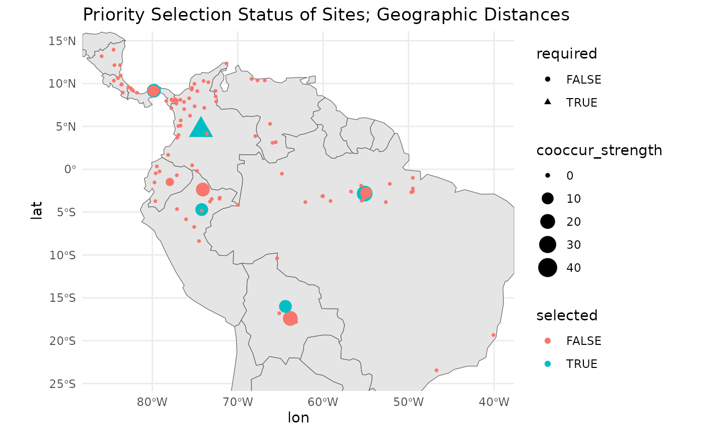
As you can see, a couple of alternative sites in very close proximity to the selected sites also score highly. These alternatives could be used as substitutes for the target sites. What is important is that these combinations are found and articulated in the results for site locations.
map +
  geom_point(data = geo_res$input_data,
    aes(
      x = lon,
      y = lat,
      shape = required,
      size = -sample_rank,
      color = sample_rank
      )
    ) +
 # ggrepel::geom_label_repel(aes(label = sample_rank), size = 4) +
theme_minimal() 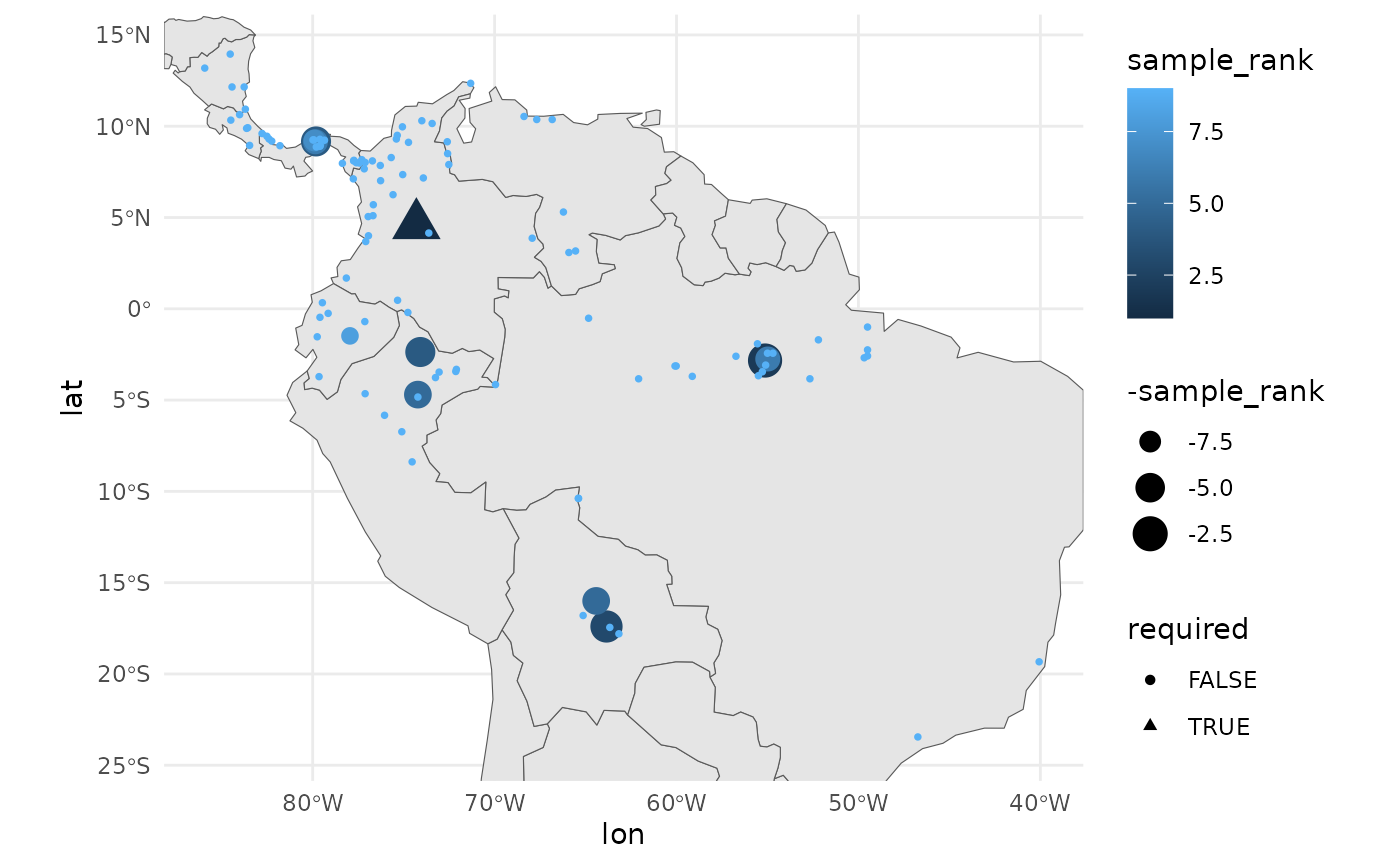
Because we believe that as many populations as possible should be sampled, we include a ‘priority’ ranking with the results. The focus should be on the selected sites, but opportunities to sample beyond them should not be overlooked.
run KMedoidsBasedSample with environmental distances
As mentioned, instead of using geographic distance, we can use environmental distance, which is ordinated in a two-dimensional space. An analyst should only consider variables they know are relevant to the species distribution for this purpose. However, for the sake of the example, we will feed in the full stack of environmental variables available from the dismo package.
extract prep environmental distances
First, to facilitate environmental distance calculations, we read in the required raster layers.
files <- list.files(
  path = file.path(system.file(package="dismo"), 'ex'),
  pattern = 'grd',  full.names=TRUE )
predictors <- terra::rast(files) # import the independent variables
rm(files)
For our environmental distances, we will use a PCA transformation of the environmental variables. We will sample 100 random points from the raster layers to calculate the PCA, and then predict the PCA raster layers across the entire study area. We will take only the first two layers from the PCA and calculate environmental distances based on them.
pts <- terra::spatSample(predictors, 100, na.rm = TRUE)
pts <- pts[, names(pts)!='biome' ] # remove categorical variable for distance calc

pca_results <- stats::prcomp(pts, scale = TRUE)
round(pca_results$sdev^2 / sum(pca_results$sdev^2), 2) # variance explained
[1] 0.58 0.23 0.11 0.05 0.02 0.00 0.00 0.00
pca_raster <- terra::predict(predictors, pca_results)
From the above, we see that the first two PCA axes account for a large portion of the variance observed in this landscape.
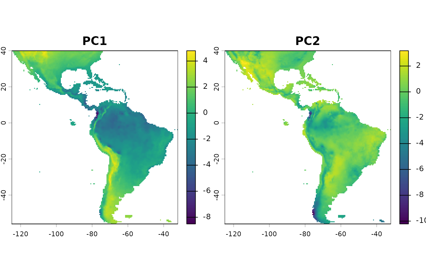
We keep the first two PCA layers for calculating the environmental distance. Including more layers increases dimensionality and may reduce the usefulness of the results. Note that it’s fine to use a Euclidean distance calculation for these, as the values are truly in the position of the pca plot.
env_values <- terra::extract(pca_raster,
  sf::st_coordinates(
    sf::st_as_sf(
      df,
      coords = c('lon', 'lat'),
      crs = 4326
    )
  )
)[,1:2]
plot(env_values, main = 'environmental distance of points from first two PCA axis')
We’ll ensure that these data are in a proper matrix format for feeding into the function.
Similar to the above run with geographic distances, we create our input object and run the function.
test_data <- list(
  distances = env_dist_mat,
  sites = df
  )

st <- system.time(
  {
    env_res <- KMedoidsBasedSample(  ## reduce some parameters for shorter run time.
      input_data = test_data,
      n = 5,
      n_bootstrap = 10,
      dropout_prob = 0.1,
      n_local_search_iter = 50,
      n_restarts = 2
    )
  }
)
Sites: 116 | Seeds: 1 | Requested: 5 | Coord. Uncertain: 19 | BS Replicates: 10
  |                                                                              |                                                                      |   0%  |                                                                              |=======                                                               |  10%  |                                                                              |==============                                                        |  20%  |                                                                              |=====================                                                 |  30%  |                                                                              |============================                                          |  40%  |                                                                              |===================================                                   |  50%  |                                                                              |==========================================                            |  60%  |                                                                              |=================================================                     |  70%  |                                                                              |========================================================              |  80%  |                                                                              |===============================================================       |  90%  |                                                                              |======================================================================| 100%

rm(dist_mat, env_dist_mat)
This run takes longer than the runs with only the geographic distance matrix.
knitr::kable(st)| x | |
|---|---|
| user.self | 34.550 |
| sys.self | 0.002 |
| elapsed | 34.554 |
| user.child | 0.000 |
| sys.child | 0.000 |
The environmental distance run takes about 10 seconds longer.
| x |
|---|
| 0.2 |
The overall stability score is similar to that of the geographic score. When you view the plots, you will see that a handful of sites in close proximity to the selected sites would have served as nearly equivalent substitutes. A few areas have dropped out of priority sampling based on this method, but in general, the results are pretty similar - the relationship between geographic and environmental distance is somewhat strong in this landscape.
map +
  geom_point(data = env_res$input_data,
    aes(
      x = lon,
      y = lat,
      shape = required,
      size = cooccur_strength,
      color = selected
      )
    ) +
 # ggrepel::geom_label_repel(aes(label = site_id), size = 4) +
  theme_minimal() +
  labs(title = 'Priority Selection Status of Sites; Environmental')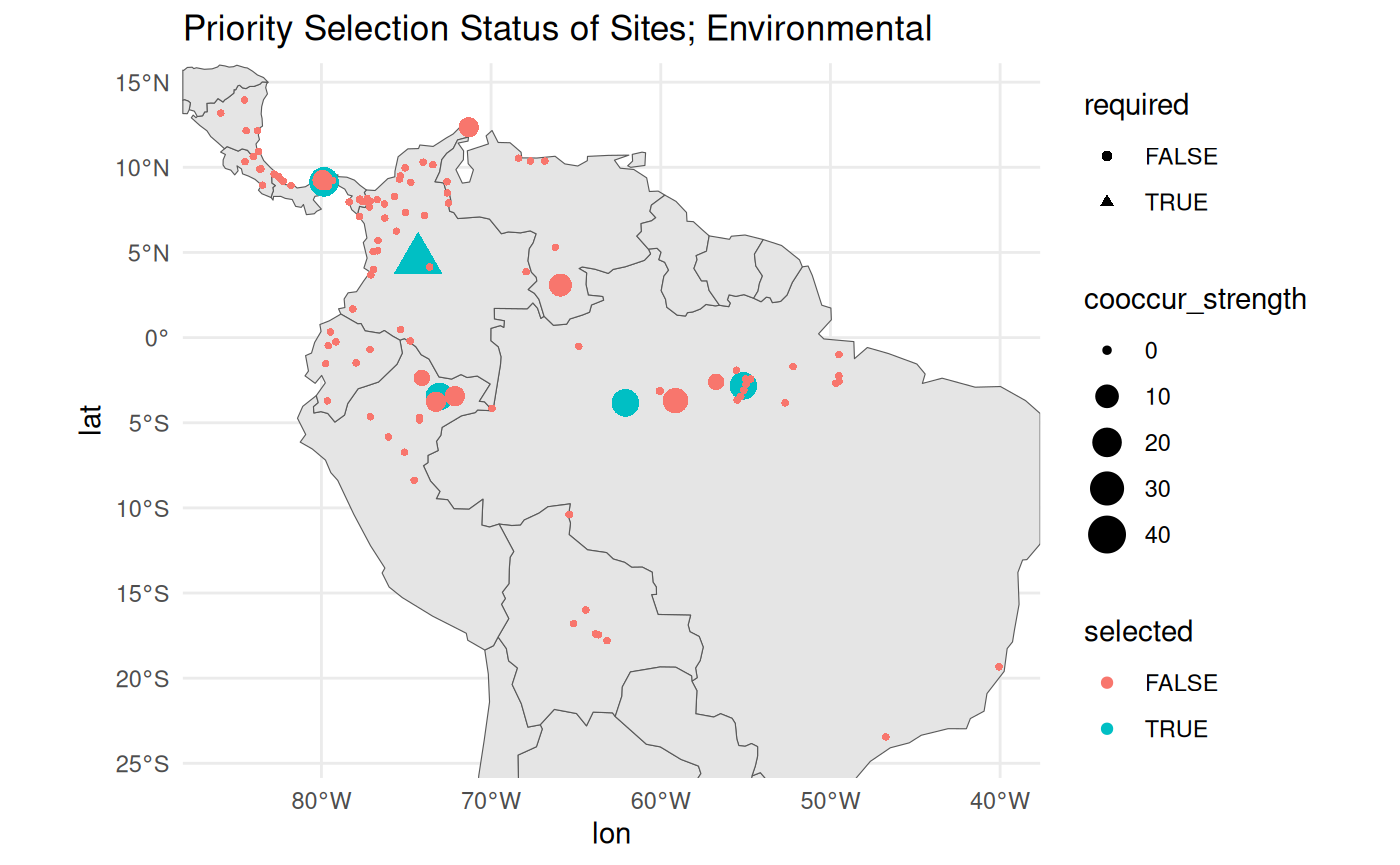
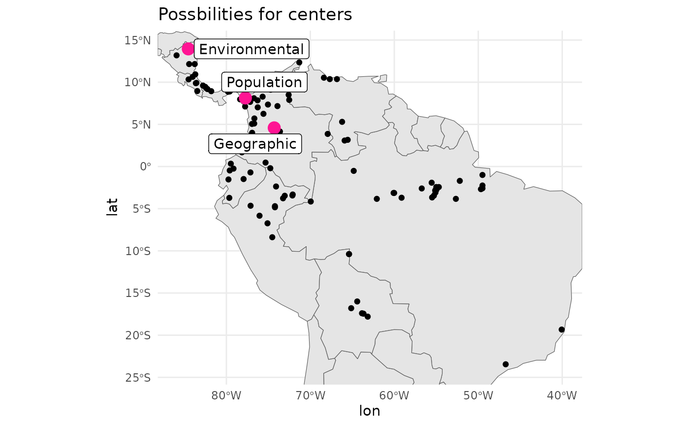
alternative methods for required central points
In the example above, we use a point at the median geographic centre of the population.
We can also identify the population with the highest population density. Intuitively, this would suggest a population with high genetic diversity for the species, although it is unlikely to have accumulated substantial local changes, as the effects of drift are overcome by more frequent dispersal.
dens <- with(df, MASS::kde2d(lon, lat, n = 200))
max_idx <- which(dens$z == max(dens$z), arr.ind = TRUE)[1,]
max_point <- c(dens$x[max_idx[1]], dens$y[max_idx[2]])

pops_centre <- sweep(df[c('lon', 'lat')], 2, max_point, "-")
pop_centered_id <- which.min(rowSums(abs(pops_centre^2)))

rm(dens, max_idx, max_point, pops_centre)
Alternatively, we can identify the population which is closest to the ‘centre’ of the environmental variable space.
env_centered <- sweep(env_values, 2, sapply(env_values, median), "-")
env_centered_id <- which.min(rowSums(abs(env_centered^2)))

rm(env_values)
Personally, I would consider the ‘pop-centred’ population to be the most important site to centre a design. However, it can suffer from sampling bias, and you may want to check that the recorded populations are deduplicated to account for this.
# geographic centroid was pt 47
centers <- df[ c(env_centered_id, pop_centered_id, 47), ]
centers$type <- c('Environmental', 'Population', 'Geographic')

map +
  geom_point(
    data = df,
    aes(x = lon, y = lat)
    ) +
  geom_point(
    data = centers,
    aes(x = lon, y = lat),
    col = '#FF1493', size = 4
    ) +
 # ggrepel::geom_label_repel(
 #   data = centers,
 #   aes(label = type, x = lon, y = lat)
 #   ) +
  theme_minimal() +
  labs(title = 'Possbilities for centers')