Overview
We have already shown that beta-coefficients from species
distribution models can be used in hierarchical clustering to group
species populations into clusters that are more similar and better
aligned with their ecology and climate. While running
EnvironmentalBasedSample, we also focus on optimising the
species-occupied range using Moran eigenvector matrix surfaces (MEMs, or
PCNMs). In this alternative approach, we drop the PCNMs from the SDMs,
focus solely on environmental predictors, identify clusters in the
current environmental space, and then classify
future environmental (and geographic) space using these
cluster parameters. This gives us sets of areas with populations that
may be more pre-adapted to future conditions. In addition to
transferring the realised environmental clusters of populations forward,
we also identify novel climate spaces, using MESS (Elith 2010) and
hierarchical clustering. This results in n identified clusters, and we
can traverse the clustering branches to determine which existing
clusters are most similar to the novel clusters.
This is the sole workflow in safeHavens that seeks to
link current climates to future scenarios, directly suggest how the size
of clusters may change and where they will shift, and allow a germplasm
curator to identify relevant seed sources for predictive provenancing.
The approach employed here is adequate to guide current collections;
decisions on which sources to use at a particular restoration site are
relatively well defined by tools such as the Seed Lot Selection Tool in
North America.
Analysis
This workstream leans heavily on the
EnvironmentalBasedSample workflow and passes its final
objects off to PolygonBasedSample for completion. Please
review Species Distribution Models and
Getting Started before proceeding here. ### Data prep
This workflow will require the geodata package;
geodata is used to retrieve climate data from various
sources as raster data. In this vignette, we will use Worldclim. For most safeHavens
users worldwide, this may be your ideal source of climate data.
geodata is developed and maintained by Robert Hijman,
similar to terra, and dismo, which are doing a
ton of heavy lifting internally on our functions.
library(safeHavens)
library(sf) ## vector operations
library(terra) ## raster operations
library(geodata) ## environmental variables
library(dplyr) ## general data handling
library(tidyr) ## general data handling
library(ggplot2) ## plotting
library(patchwork) ## multiplots
set.seed(22)
For this example, we will leverage GBIF data and shift our geographic focus to the Colorado Plateau in the Southwestern USA. The Colorado Plateau is predicted to experience some of the highest rates of climate change on the planet, and is already an area with considerable native seed development activities. For our focal species, we will use Helianthella microcephala for no other reason than that it exists in relatively homogenous portions of the Colorado Plateau - meaning we can download relatively coarse rasters for the vignettes, and that it has a stunning inflorescence.
cols = c('decimalLatitude', 'decimalLongitude', 'dateIdentified', 'species', 'acceptedScientificName', 'datasetName',
  'coordinateUncertaintyInMeters', 'basisOfRecord', 'institutionCode', 'catalogNumber')

## download species data using scientificName, can use keys and lookup tables for automating many taxa.
hemi <- rgbif::occ_search(scientificName = "Helianthella microcephala")
hemi <- hemi[['data']][,cols]  |>
  drop_na(decimalLatitude, decimalLongitude) |> # any missing coords need dropped.
  distinct(decimalLatitude, decimalLongitude, .keep_all = TRUE) |> # no dupes can be present
  st_as_sf(coords = c( 'decimalLongitude', 'decimalLatitude'), crs = 4326, remove = F)

western_states <- spData::us_states |> ## for making a quick basemap.
  dplyr::filter(NAME %in%
    c('Utah', 'Arizona', 'Colorado', 'New Mexico', 'Wyoming', 'Nevada', 'Idaho', 'California')) |>
  dplyr::select(NAME, geometry) |>
  st_transform(4326)

bb <- st_bbox(
  c(
    xmin = -116,
    xmax = -105,
    ymax = 44,
    ymin = 33.5),
    crs = st_crs(4326)
    )

western_states <- st_crop(western_states, bb)
Warning: attribute variables are assumed to be spatially constant throughout
all geometries

bmap <- ggplot() +
    geom_sf(data = western_states) +
    geom_sf(data = hemi) +
    theme_minimal() +
    coord_sf(
        xlim = c(bb[['xmin']], bb[['xmax']]),
        ylim = c(bb[['ymin']], bb[['ymax']])
        )  +
    theme(
      axis.title.x=element_blank(),
      axis.text.x=element_blank(),
      axis.ticks.x=element_blank()
      )

bmap +
    labs(title = 'Helianthella microcephala\noccurrence records')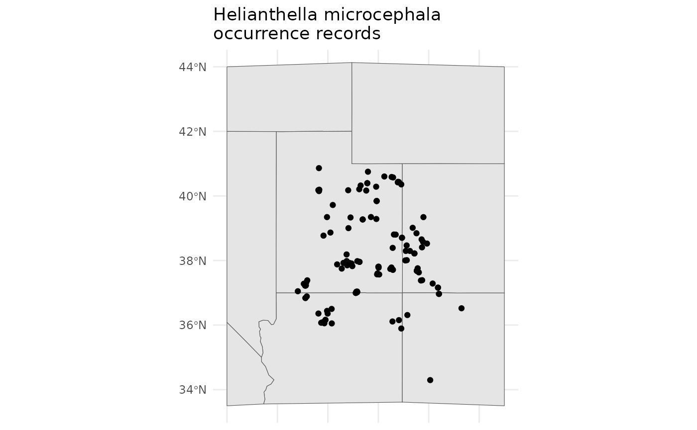
We will download WorldClim data using geodata. The
results from worldclim_global should match what we loaded
from dismo in the various sloth examples. For our future scenario, we
will use the CMIP6 modelled
future climate data for the 2041-2060 time window. We will download the
coarse 2.5-minute resolution data, ca. ~70km at the equator. Do note
that the source also includes a ~1km at-equator resolution data set (30
seconds), but this would take too long for the vignette.
# Download WorldClim bioclim at ~10 km
bio_current <- worldclim_global(var="bioc", res=2.5)
Cached as: /tmp/RtmpNl2gVK/climate/wc2.1_2.5m//wc2.1_2.5m_bio.zip
bio_future <- cmip6_world(
  model = "CNRM-CM6-1", ## modelling method
  ssp   = "245", ## "Middle of the Road" scenario
  time  = "2041-2060", # time period
  var   = "bioc", # just use the bioclim variables
  res   = 2.5
)
Cached as: /tmp/RtmpNl2gVK/climate/wc2.1_2.5m//wc2.1_2.5m_bioc_CNRM-CM6-1_ssp245_2041-2060.tif

# Crop to domain - use a large BB to accomodate range shift
# under future time points.
# but going too large will dilute the absence records
bbox <- ext(bb)

bio_current <- crop(bio_current, bbox)
bio_future <- crop(bio_future, bbox)
safeHavens does not provide explicit functionality to
rename / align raster surface naming. However, the modelling process
requires that both current and future raster products have perfectly
matching raster names.
The chunk below shows how we will standardise the names by extracting the bioclim variable number at the end of the name and padding ‘bio_’ back to the front with a leading zero, so we have ‘bio_01’ instead of ‘bio_1’. A minor variation of this should work for most data sources, after customising the gsub to erase earlier portions of the file name.
simplify_names <- function(x){
    paste0('bio_', sprintf("%02d", as.numeric(gsub('\\D+','', names(x)))))
}

names(bio_current) <- gsub('^.*5m_', '', names(bio_current))
names(bio_future) <- gsub('^.*2060_', '', names(bio_future))

names(bio_current) <- simplify_names(bio_current)
names(bio_future) <- simplify_names(bio_future)

# TRUE means all names match, and are in the same position.
all(names(bio_current) == names(bio_future))
[1] TRUE

## we will also drop some variables that are essentially identical in the study area
drops <- c(
  'bio_05' , 'bio_02',
  'bio_11', 'bio_12'
  )

bio_current <- subset(bio_current, negate = TRUE, drops)
bio_future <- subset(bio_future, negate = TRUE, drops)
If you are following the vignette locally, you will find that
plot(bio_current) and plot(bio_future) look
very similar. While the plots look very similar when showing one raster
stack after another, we can diff the two products to see where the
largest changes occur in geographic space.
pct_diff <- function(x, y){((x - y)/((x + y)/2)) * 100}
difference <- pct_diff(bio_current, bio_future)
plot(difference)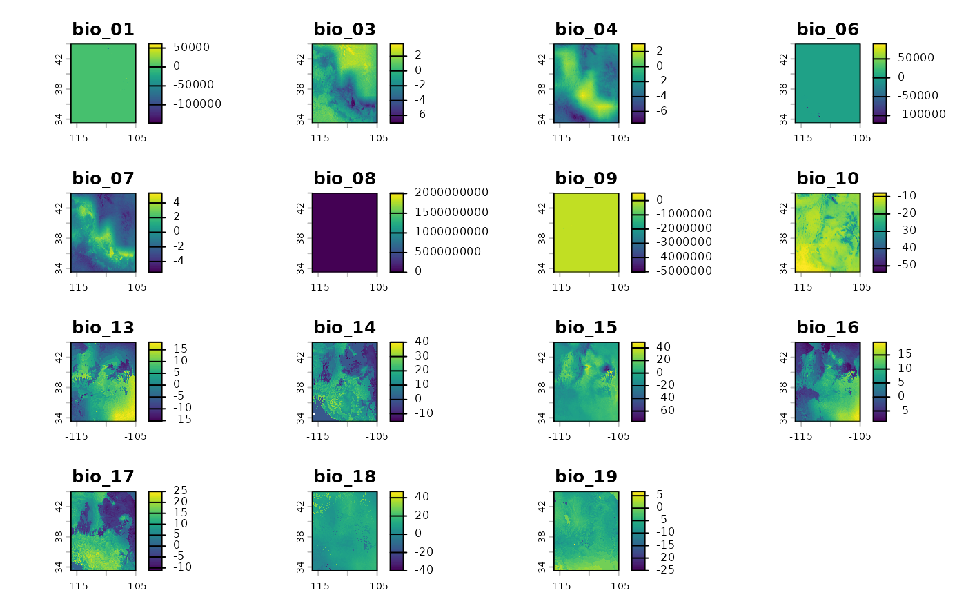
We see that variables exhibit inconsistencies in where they change and to what extent. This mismatch of conditions will almost certainly lead to novel climate conditions - unique combinations not yet known to this species. This will be handled using MESS surfaces and a second-stage clustering approach in the function.
Analytical workstream
The workflow for predictive provenance builds upon the
EnvironmentalBasedSample workflow, relying on many of the
same internal helpers and user-facing functions. Note that when using
elasticSDM, we need to specify pcnm = FALSE to
bypass fitting a model with PCNM surfaces; there is no analogue for
these in future scenarios, so they must be dropped.
Fit SDM and rescale raster surfaces
The starting point for this analysis is again fitting a quick SDM for our species.
## note we subset to just the geometries for the prediction records.
# this is because we feed in all columns to the elastic net model internally.
hemi <- select(hemi, geometry)

# as always verify our coordinate reference systems (crs) match.
st_crs(bio_current) == st_crs(hemi)
[1] TRUE

# and fit the elasticnet model
eSDM_model <- elasticSDM(
    x = hemi,
    predictors = bio_current,
    planar_projection = 5070,
    PCNM = FALSE ## set to FALSE for this workstream!!!!!
    )
We will use the eSDM_model function for this workstream; however, it is essential that PCNM is set to FALSE. There is no way to forecast or predict PCNM for future scenarios, so we cannot fit models with it.
If a warning is emitted here, it is likely due to collinearity in the
bioclim variables. The function will internally dro- collinear
predictors to try and maintain eDist usage (just for this
step), but if this fails will fall back to the eRandom method
instead.
knitr::kable(eSDM_model$ConfusionMatrix$byClass[
c('Sensitivity', 'Specificity', 'Recall', 'Balanced Accuracy')])| x | |
|---|---|
| Sensitivity | 0.9615385 |
| Specificity | 0.6923077 |
| Recall | 0.9615385 |
| Balanced Accuracy | 0.8269231 |
plot(eSDM_model$RasterPredictions)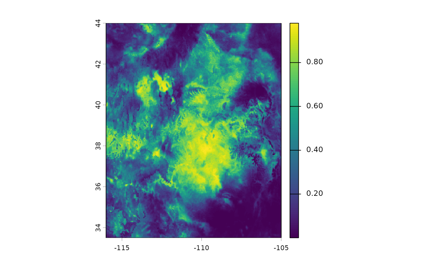
We can view some of the model results; they are OK, but would benefit
from using only a subset of the bioclim predictors to allow for
eDist sampling upstream. It is a bit too generous in
classifying areas as being possibly suitable habitat. While this model
would be unsuitable for applications, certain CRAN and GitHub checks
make it difficult to improve upon as an example.
Using the beta coefficients from the model, we will rescale both the current and future climate scenario rasters. This will happen internally in the next function, but it is good to see the difference between the current and future scenarios to have an idea of expectations for the final results.
bio_current_rs <- RescaleRasters(
    model = eSDM_model$Model,
    predictors = eSDM_model$Predictors,
    training_data = eSDM_model$Train,
    pred_mat = eSDM_model$PredictMatrix
    )

plot(bio_current_rs$RescaledPredictors)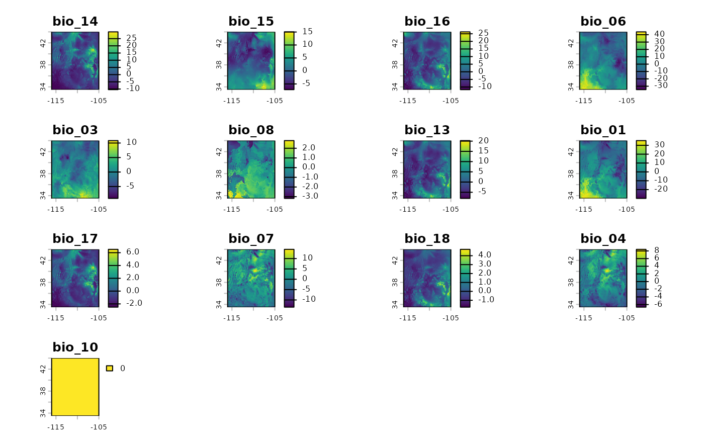
bio_future_rs <- rescaleFuture(
  eSDM_model$Model,
  bio_future,
  eSDM_model$Predictors,
  training_data = eSDM_model$Train,
  pred_mat = eSDM_model$PredictMatrix
)

plot(bio_future_rs)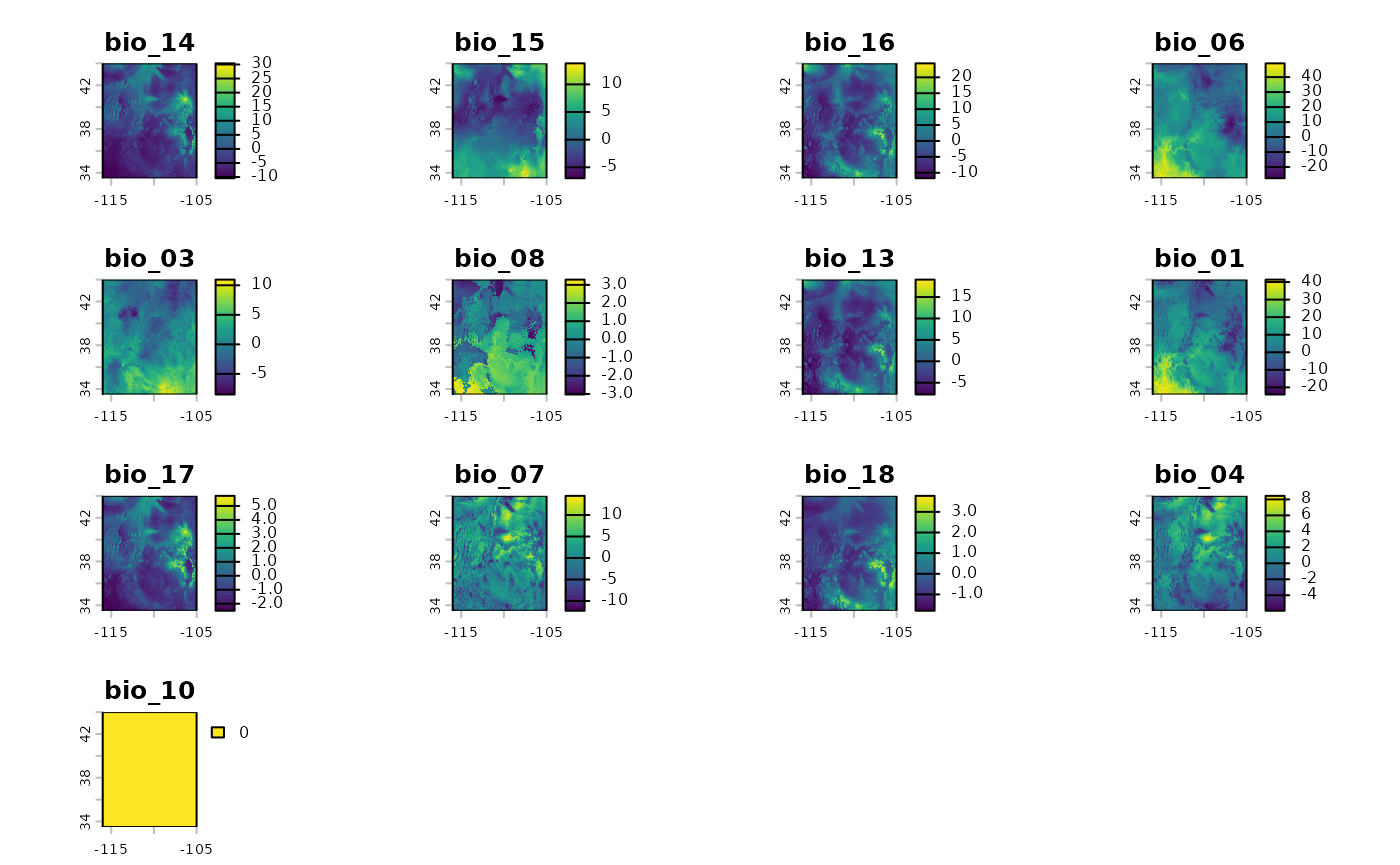
If any of the layers show as a single colour and 0, it means that glmnet shrunk them out of the model.
Similar to how we differenced the rasters at the two time points above, we can take the absolute difference between the relevant raster layers to see where the largest changes occur.
difference_rs <- pct_diff(bio_current_rs$RescaledPredictors, bio_future_rs)
plot(difference_rs)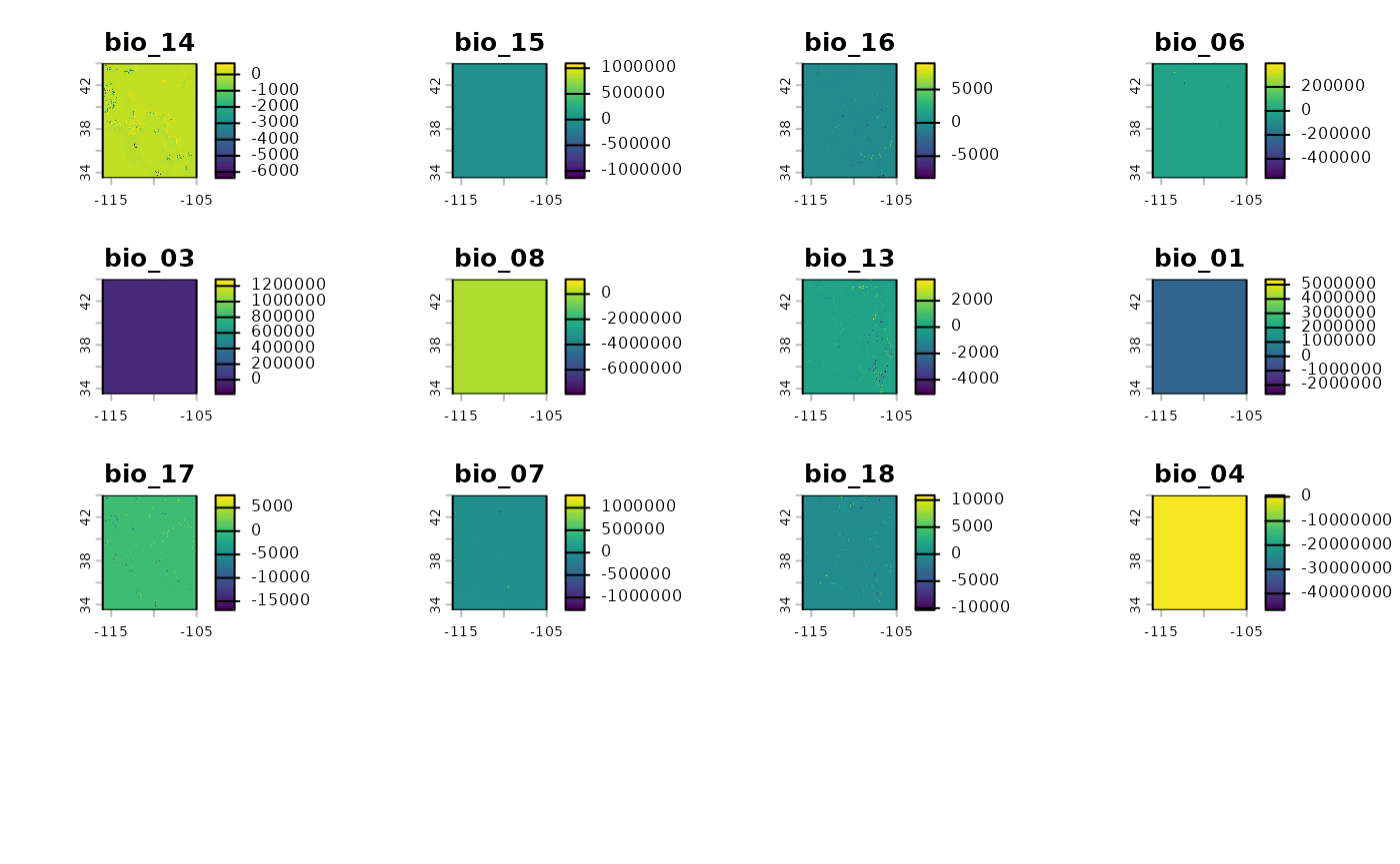
The above plot shows us the areas with the largest changes between current and predicted conditions.
Cluster surfaces
Clusters can be identified using NbClust, which determines the
optimal n using the complete consensus method. To use
NbClust, rather than manually specifying n, the argument
fixedClusters needs to be set to FALSE. When using
PostProcessSDM, the same thresh metric should
be used as the one applied to PredictiveProvenance.
threshold_rasts <- PostProcessSDM(
  rast_cont = eSDM_model$RasterPredictions,
  test = eSDM_model$TestData,
  train = eSDM_model$TrainData,
  planar_proj = 5070,
  thresh_metric =
     'equal_sens_spec',
  quant_amt = 0.25
  )

plot(threshold_rasts$FinalRasters)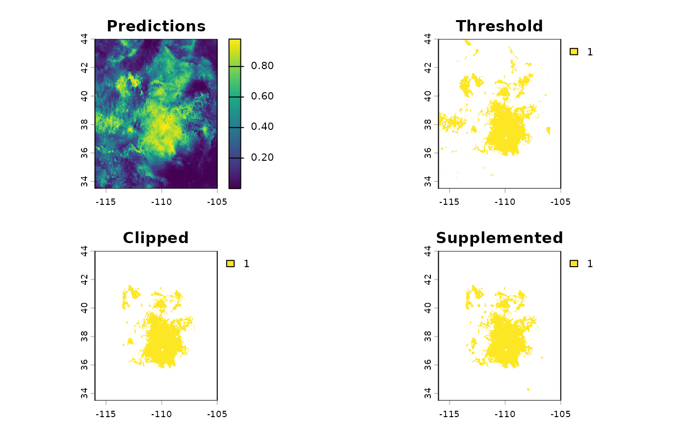
knitr::kable(threshold_rasts$Threshold$equal_sens_spec)| x |
|---|
| 0.6162985 |
bmap +
  geom_sf(data =
  sf::st_as_sf(
    terra::as.polygons(
      threshold_rasts$FinalRasters['Threshold'])
      ), fill = 'cornsilk'
    ) +
geom_sf(data = hemi) 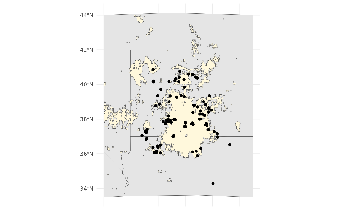
We will use the EnvironmentalBasedSample to determine a
suitable number of climate clusters for the current time period. When
using EBS for predictive provencing also set the coord_wt
parameter to a small value. This will remove the effect of the spatial
clustering. Similar to PCNM, we cannot know the distribution of actual
populations in the future.
ENVIbs <- EnvironmentalBasedSample(
  pred_rescale = bio_current_rs$RescaledPredictors,
  write2disk = FALSE, # we are not writing, but showing how to provide some arguments
  f_rasts = threshold_rasts$FinalRasters,
  coord_wt = 0.001,
  fixedClusters = FALSE,
  lyr = 'Threshold',
  n_pts = 500,
  planar_proj = "epsg:5070",
  buffer_d = 3,
  prop_split = 0.8,
  min.nc = 5,
  max.nc = 15
  )
bmap +
  geom_sf(data = ENVIbs$Geometry, aes(fill = factor(ID))) +
  geom_sf(data = hemi) +
  theme(legend.position = 'bottom') +
  labs(fill = 'Cluster', title = 'Current')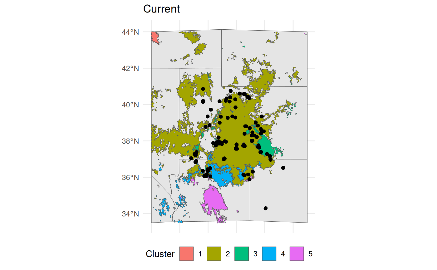
We can apply the current clustering to the future scenario. This will
show us how and where the currently identified clusters would exist in
the future geographic space. ProjectClusters is really the
heart of this workflow; it requires the outputs from
elasticSDM, PostProcessSDM, and
EnvironmentalBasedSample.
future_clusts <- projectClusters(
  eSDM_object = eSDM_model,
  current_clusters = ENVIbs,
  future_predictors = bio_future,
  current_predictors = bio_current,
  thresholds = threshold_rasts$Threshold,
  planar_proj = "epsg:5070",
  thresh_metric = 'equal_sens_spec',
  n_sample_per_cluster = 20
)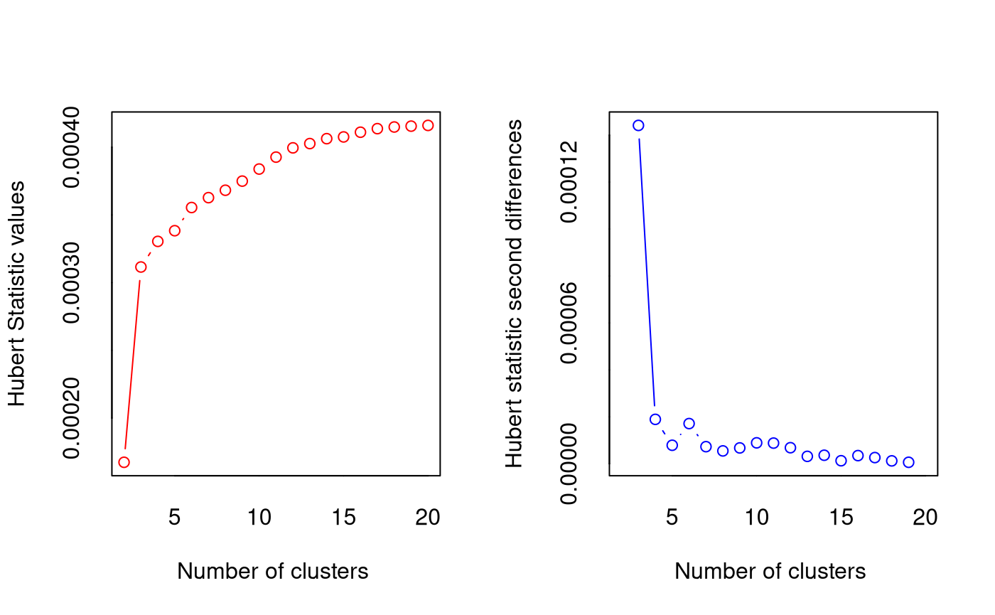
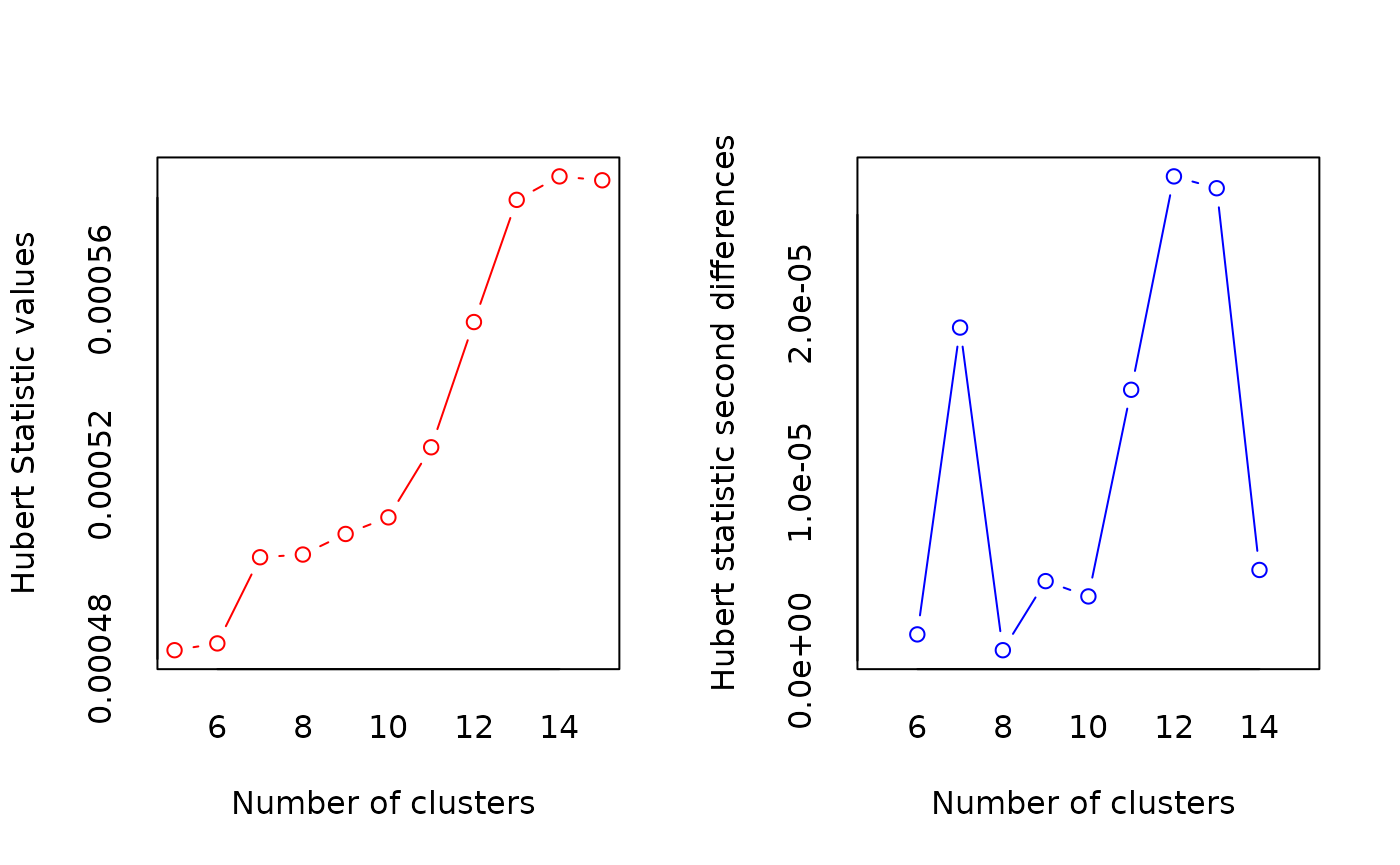
*** : The Hubert index is a graphical method of determining the number of clusters.
                In the plot of Hubert index, we seek a significant knee that corresponds to a
                significant increase of the value of the measure i.e the significant peak in Hubert
                index second differences plot.
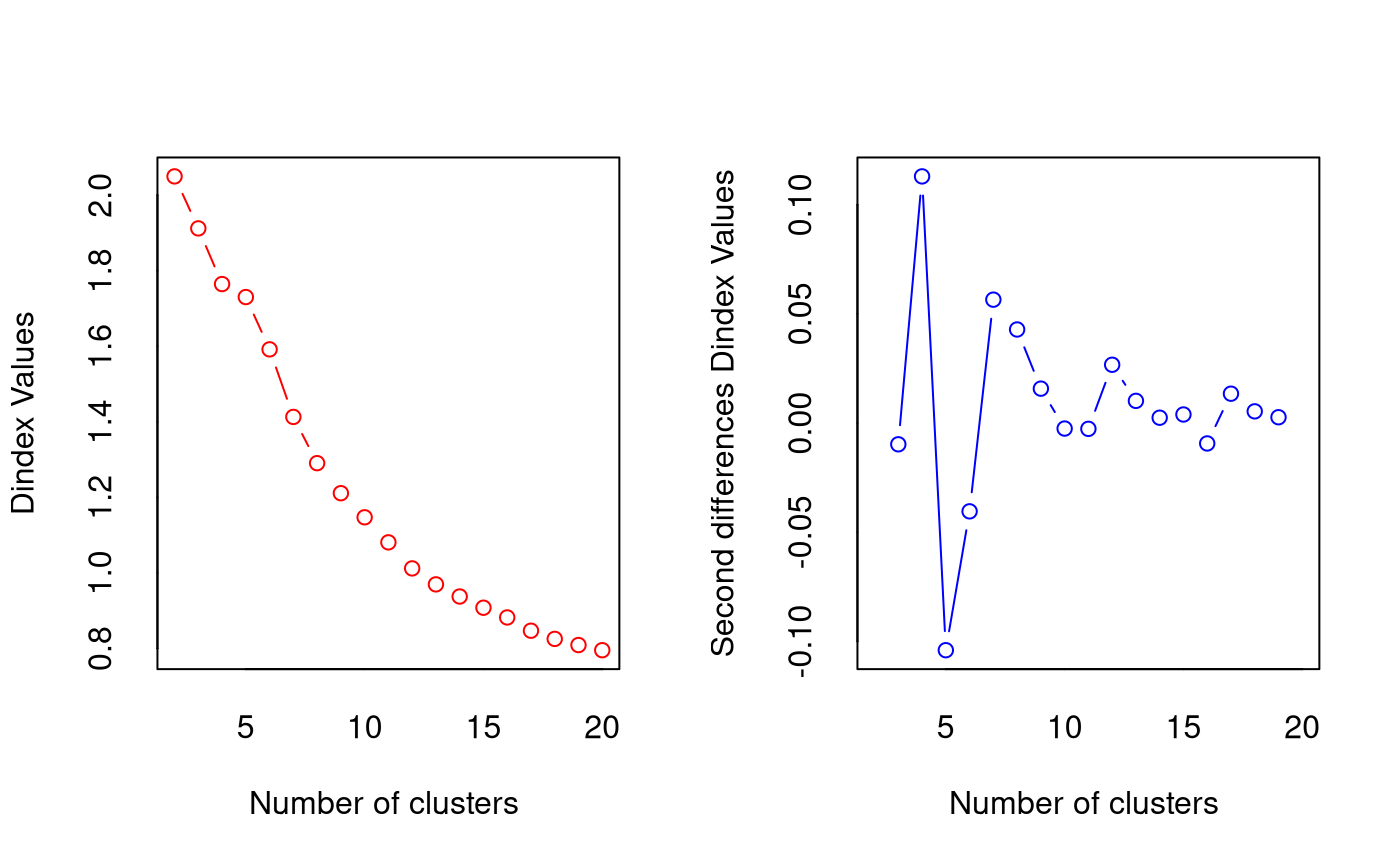
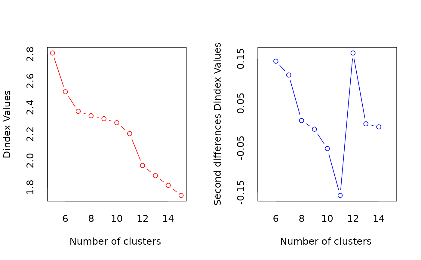
*** : The D index is a graphical method of determining the number of clusters.
                In the plot of D index, we seek a significant knee (the significant peak in Dindex
                second differences plot) that corresponds to a significant increase of the value of
                the measure.

*******************************************************************
* Among all indices:
* 1 proposed 2 as the best number of clusters
* 16 proposed 3 as the best number of clusters
* 3 proposed 4 as the best number of clusters
* 1 proposed 10 as the best number of clusters
* 1 proposed 19 as the best number of clusters
* 1 proposed 20 as the best number of clusters

                   ***** Conclusion *****

* According to the majority rule, the best number of clusters is  3


*******************************************************************
However, our classifications cannot accommodate new climate conditions. We can identify these areas outside the training conditions for our SDM using MESS. Note that in these areas, our SDM is extrapolating, so its performance cannot be evaluated. However, it seems these may be suitable habitats, and we can plan for that scenario.
plot(future_clusts$mess)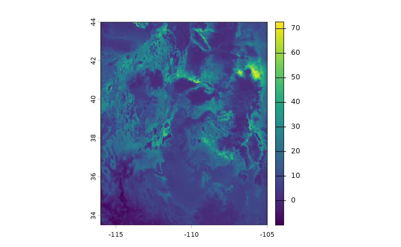
bmap +
  geom_sf(data =
    st_as_sf(terra::as.polygons(future_clusts$novel_mask)),
    fill = 'red') +
  labs(title = 'MESS regions')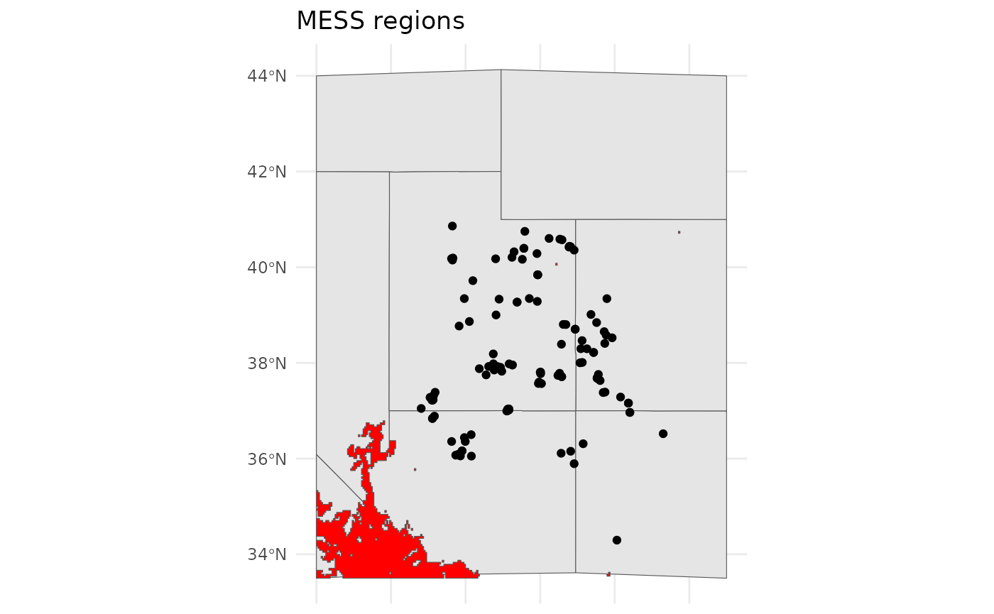
Once we identify these areas, if they are sufficiently large, we can pass them to a new NbClust scenario, and it can cluster them anew.
current = bmap +
  geom_sf(data = ENVIbs$Geometry, aes(fill = factor(ID))) +
  labs(title = 'Current', fill = 'Cluster') +
  theme(legend.position = "none")

future = bmap +
  geom_sf(data = future_clusts$clusters_sf, aes(fill = factor(ID))) +
  labs(title = '2041-2060', fill = 'Cluster')

current + future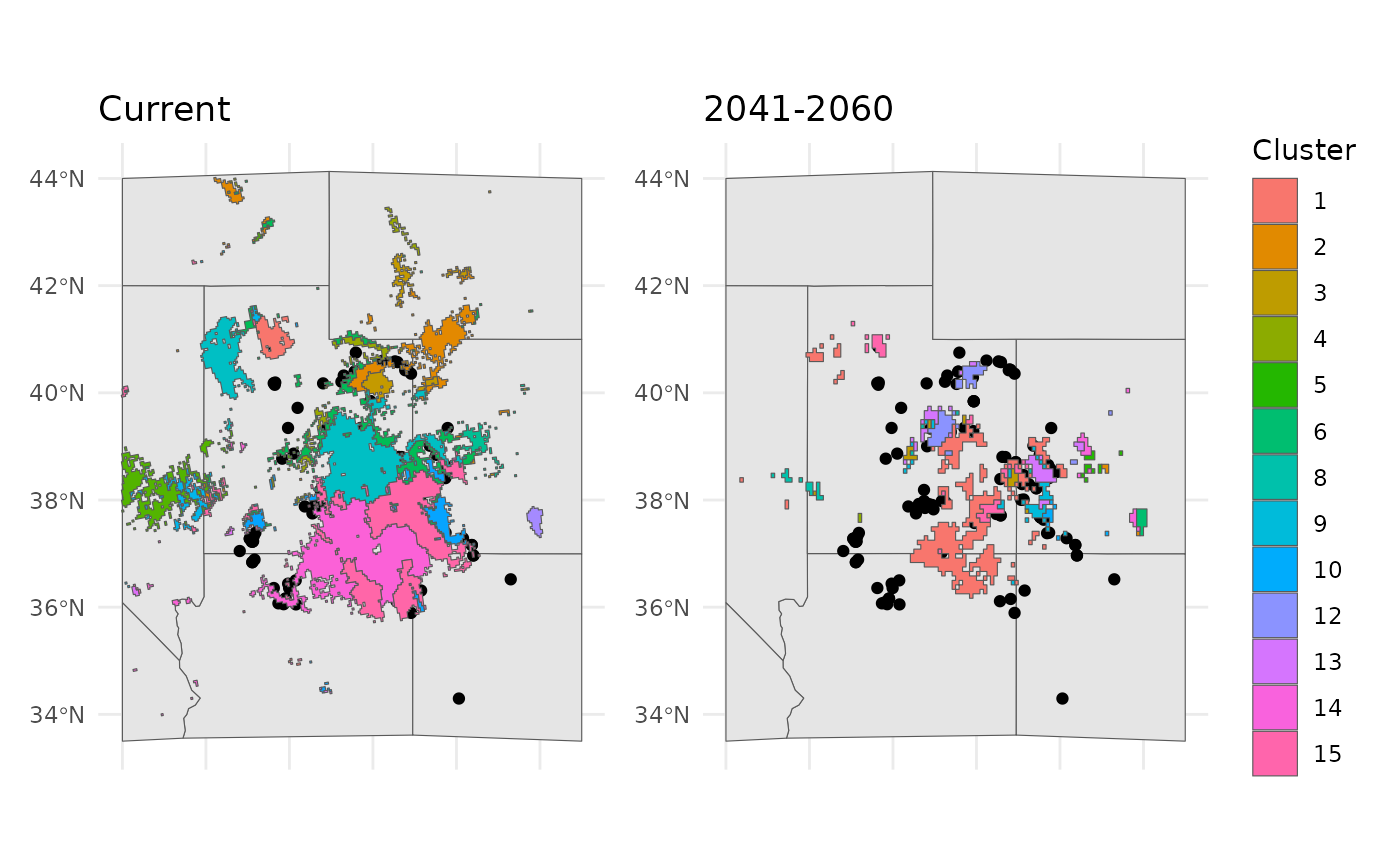
However, we also need to determine which current areas are most similar to these novel climate clusters. We can take values from both classifcation scenarios, cluster them, and identify which new climate clusters share branches with existing clusters. This is the method we employ to identify the most similar existing climate groups.
knitr::kable(future_clusts$novel_similarity)| novel_cluster_id | nearest_existing_id | avg_silhouette_width |
|---|---|---|
| 11 | 5 | 0.4864734 |
| 12 | 3 | 0.3681229 |
It is from these groups that we are most likely to collect germplasm relevant to the future scenarios.
We can also take a very quick look at how cluster sizes change between the scenarios.
future_clusts$changes
   cluster_id current_area_km2 future_area_km2 area_change_pct
1           1        5391.0984       4803.1331       -10.90622
2           2         631.2362        945.9330        49.85405
3           3       64079.0045      78281.8787        22.16463
4           4       57903.1260      41211.1558       -28.82741
5           5        9332.0595      31687.7516       239.55797
6           6        9059.0925      41998.2457       363.60323
7           7       53638.0165        353.5715       -99.34082
8           8       48554.0061       4436.8433       -90.86204
9           9        7864.8618       9585.4532        21.87694
10         10        1450.1372        692.1030       -52.27328
11         11           0.0000       4174.1658              NA
12         12           0.0000       7062.7577              NA
   centroid_shift_km
1          276.90811
2           10.05054
3          399.87854
4          668.67220
5          383.06873
6          283.93753
7          319.77316
8          859.06211
9          450.05435
10         453.36474
11                NA
12                NA
Conclusion
All functions in safeHavens work to identify areas where
populations have the potential to maximise the coverage of neutral and
allelic (genetic) diversity across the species. Large-scale restoration
requires the availability of seed sources and funding opportunities to
use them. Developing germplasm materials from populations that seem
adapted to future climate conditions is essential for future
opportunities. While this function does not in any way seek to identify
the best available seed source for a restoration, ala SST, it does seek
to ensure that the best available option can be applied in a timely
manner as the occasion arises.
This is particularly important for areas that cannot plan restorations or develop their own seed sources using point-based analyses.