Isolation by Resistance Sampling
Landscape genetics has laddered null hypotheses regarding the genetic structure of species. The first null, Panmixia, is that populations show no differentiation, as could be observed in a species with few, highly connected populations; this package does not treat it as a sampling scenario. The second null is Isolation by Distance, the main idea behind most of the functions in this package, in which populations become more differentiated with increasing geographic distance, culminating in the function ‘IBDBasedSample’.The next hypothesis is Isolation by Resistance, where the differentiation of populations is driven by a break down in gene flow due to barriers.
While IBD is easily calculated from geographic distances, IBR requires a parameterised cost surface, in raster format, that depicts the costs to an organism’s movement of maternal and paternal genetic material. safeHavens supports a simple workflow for parameterising a cost surface that can be used for basic IBR-type sampling.
Example
We’ll use the species occurrence data from dismo again here. A few spatial data sets suitable for nearly all users’ IBR applications are included in safeHavens for this example, but the full data sets are not shipped with the package.
They include: - lakes, Lehner et al. 2025, GLWD
- oceans from Natural Earth, https://www.naturalearthdata.com/downloads/10m-physical-vectors/
- rivers from FAO,
- tri (terrain ruggedness index), Amatulli et al. 2018, https://www.earthenv.org/topography
library(safeHavens)
library(sf) ## vector operations
library(terra) ## raster operations
library(dplyr) ## general data handling
library(ggplot2) ## plotting
We’ll load the species occurrence data and make it explicitly spatial.
data prep
Each of the environmental variable data sources needs some pre-processing before being fed into the IBR workflow; most of them just need to be converted from vector to raster formats - a process we call ‘rasterisation’. We will also rescale the tri rasters to put them on a similar numeric scale to the other datasets.
tri <- terra::rast(file.path(system.file(package = "safeHavens"), "extdata", "tri.tif"))
names(tri) <- 'tri'

rescale_rast <- function(r, new_min = 0, new_max = 1) {
  r_min <- global(r, "min", na.rm = TRUE)[[1]]
  r_max <- global(r, "max", na.rm = TRUE)[[1]]
  ((r - r_min) / (r_max - r_min)) * (new_max - new_min) + new_min
}

tri <- rescale_rast(tri, 0, 100)

lakes_v <- sf::st_read(
  file.path(system.file(package = "safeHavens"),  "extdata", "lakes.gpkg"),
    quiet = T) |>
  filter(TYPE == 'Lake') |> # remove reservoirs for our purposes (time scale)
  select(geometry = geom) |>
  mutate(Value = 1) |> # this will be rasterized.
  terra::vect()

ocean_v <- sf::st_read(
  file.path(system.file(package = "safeHavens"), "extdata", "oceans.gpkg"),
   quiet = T) |>
  select(geometry = geom) |>
  mutate(Value = 1) |>
  terra::vect()

rivers_v <- sf::st_read(
  file.path(system.file(package = "safeHavens"), "extdata", "rivers.gpkg"),
   quiet = T) |>
  select(geometry = geom) |>
  mutate(Value = 1) |>
  terra::vect()
We’ll convert each of the above spatVect objects to spatRasters and clip them to an analysis area around our species records.
x_buff <- sf::st_transform(x, planar_proj) |>
  # huge buffer for the bbox.
  st_buffer(200000) |>
  st_transform(crs(lakes_v)) |>
  st_as_sfc() |>
  st_union() |>
  vect() |>
  ext()

lakes_v <- crop(lakes_v, x_buff)
rivers_v <- crop(rivers_v, x_buff)
ocean_v <- crop(ocean_v, x_buff)
tri <- crop(tri, x_buff)
Convert the vector data to raster format using terra’s
rasterise function.
ocean_r <- rasterize(ocean_v, tri, field = 'Value', background = 0.1)
lakes_r <- rasterize(lakes_v, tri, field = 'Value',  background = 0.1)
rivers_r <- rasterize(rivers_v, tri, field = 'Value',  background = 0.1)

par(mfrow=c(2, 2))
plot(rivers_r)
plot(lakes_r)
plot(ocean_r)
plot(tri)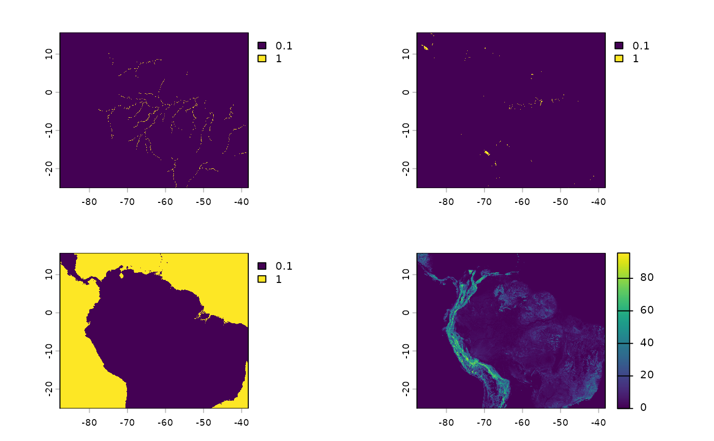
actual workflow.
The first of three functions in the Isolation by Resistance sampling
workflow is used to create the resistance surface. It requires a
template raster and the other rasters, which will be incorporated into
the product. buildResistanceSurface essentially just
requires the rasters we configured above and user-specified weights for
each raster. These weights convey how difficult it is for a species to
move across the landscape. For plants, oceans generally get very high
weights, while lakes and rivers - still obstacles - receive lower
weights. Terrain ruggedness values are much more likely to vary with
both the species’ ecology and the landscape being sampled.
When considering weights, consider the influences of bird dispersal, land animal dispersal, and natural population growth/expansion. Tuning this part is challenging and often subjective. The values below are the functions’ defaults - to my eyes, they work OK for the landscape at hand; although an ecologist with experience in this region may beg to differ, and I would not argue with them.
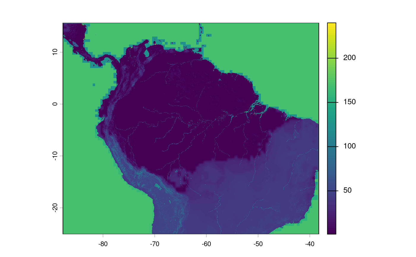
res_surface <- buildResistanceSurface(
  base_raster = rast(ocean_r), # template

  oceans = ocean_r, # rasters
  lakes = lakes_r,
  rivers = rivers_r,
  tri = tri,

  w_ocean = 120, # weights to multiple  input raster values by --
  w_lakes = 50, # is 1 * 50
  w_rivers = 20, # is 1 *20
  w_tri = 4 # ranges from 1~30, so from (1-30)*4 up to a weight of ~120.
)

plot(res_surface)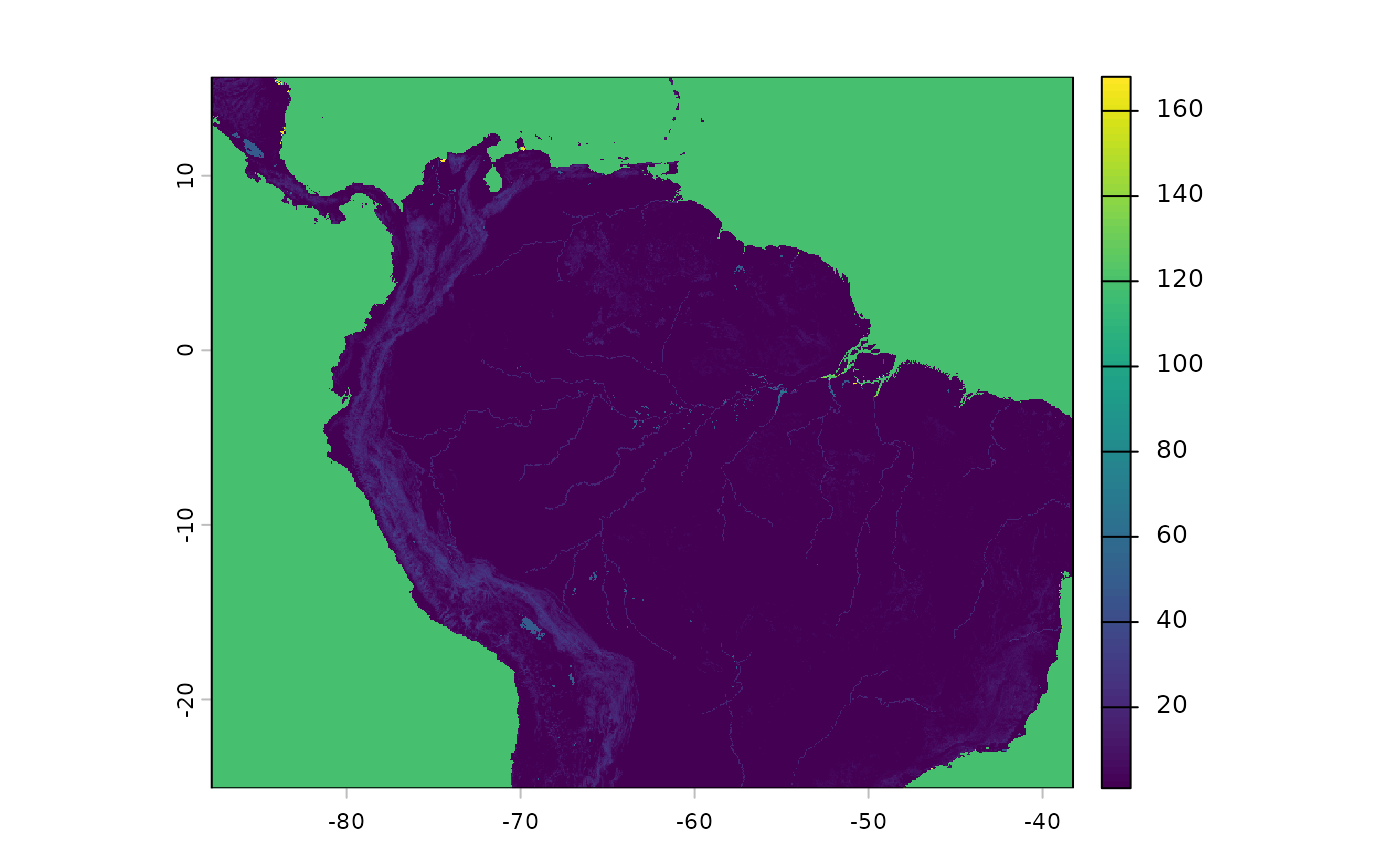
Note that the above object is stored in memory. I recommend using coarse raster surfaces (e.g., 4 km x 4 km cells or larger) at this level of generalisation and to speed up processing.
Now that we have our resistance surface, the next step is calculating
the distances between areas across the species range using the function
populationResistance. Similar to other functions in
safeHavens we will not use population occurrence record
data directly, as we know that spatial biases affect occurrence record
distributions. Rather we will buffer (buffer_dist) the
occurrence records, using a relevant planar_proj, and
create a raster surface of their locations. From this surface we will
sample n points (using terra::spatSample, with method =
‘spread’), and identify neighboring points using a
graph_method, either delauney triangulation, which is
useful when a very high n is required, or through a
complete distance matrix. In my testing I greatly prefer
results from ‘complete’ calculations, and these work with NbClust
without having to be ordinated down into 2-dimensional space and give
much better results.
This function returns a raster representing the buffered populations (species range in the domain), the points sampled by terra, the graph information, and a distance matrix containing the least-cost distances from the resistance surface.
pop_res_graphs <- populationResistance(
  base_raster = rast(ocean_r),
  populations_sf = x,
  n = 150,
  planar_proj = 3857,
  buffer_dist = 125000,
  resistance_surface = res_surface,
  graph_method = 'complete'
)

names(pop_res_graphs)
[1] "pop_raster"     "sampled_points" "spatial_graph"  "edge_list"
[5] "ibr_matrix"
Buffered locations appear as shown; IDs are meaningless.
plot(pop_res_graphs$pop_raster)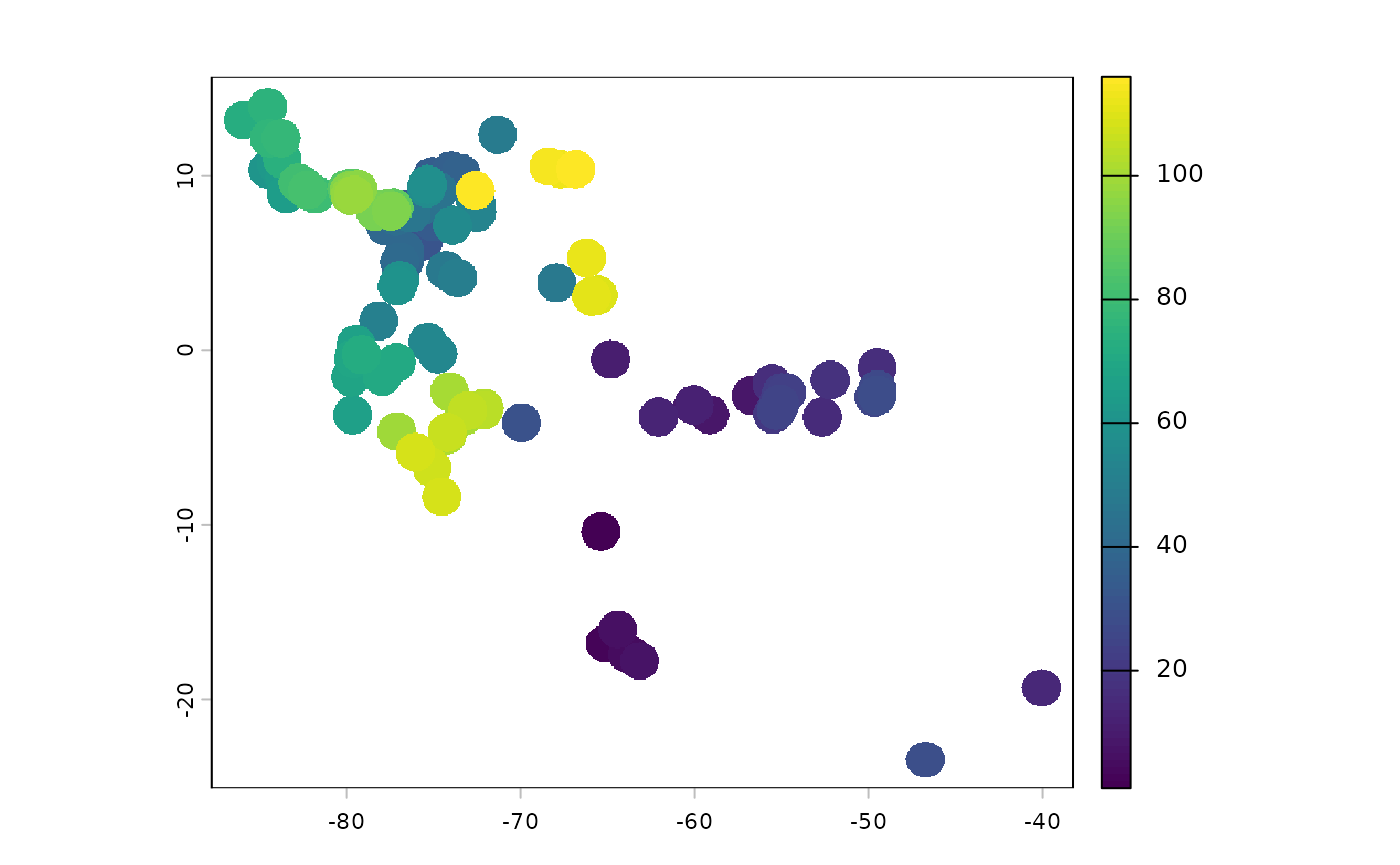
This function underperforms with user-prespecified n;
passing min.nc to NbClust generally yields the
analyst-specified value.
ibr_groups <- IBRSurface(
base_raster = rast(ocean_r),
resistance_surface = res_surface,
pop_raster = pop_res_graphs$pop_raster,
pts_sf = pop_res_graphs$sampled_points,
ibr_matrix = pop_res_graphs$ibr_matrix,
fixedClusters = TRUE,
n = 20,
planar_proj = 3857
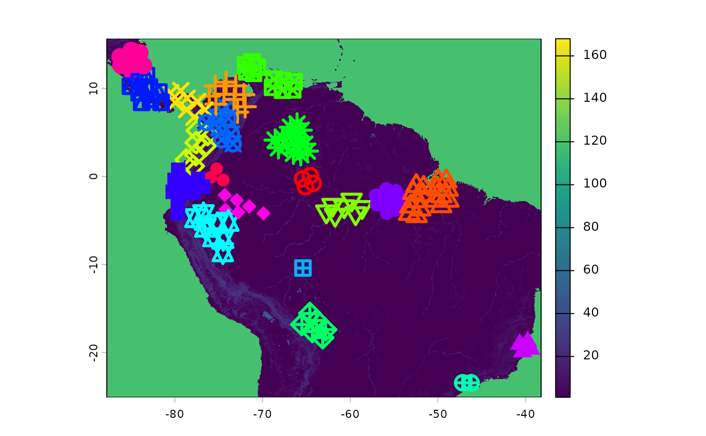
)Clustering results are shown below.
classified_pts = ibr_groups$points
plot(res_surface)
points(
  classified_pts,
  pch = as.numeric(as.factor(classified_pts$ID)),  # different symbol per ID
  col = rainbow(length(unique(classified_pts$ID)))[as.factor(classified_pts$ID)],
  cex = 2,
  lwd = 3
  )
Occupied area clusters are visualised below.
ggplot() +
  geom_sf(data = ibr_groups$geometry, aes(fill = factor(ID))) +
  theme_minimal()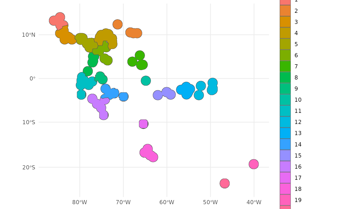
Finally, the surface can be sampled using
PolygonBasedSample. Simply union the geometries to be the
species range, and supply the groups to the x argument, in lieu of an
ecoregion or pSTZ-type surface.
out <- PolygonBasedSample(
  x = st_union(ibr_groups$geometry),
  zones = ibr_groups$geometry,
  zone_key = 'ID',
  n  = 30
  )

ggplot(data = out) +
  geom_sf(aes(fill = factor(allocation))) +
  theme_minimal() +
  labs(fill = 'Ct. collections\nper cluster') +
  theme(legend.position = 'bottom')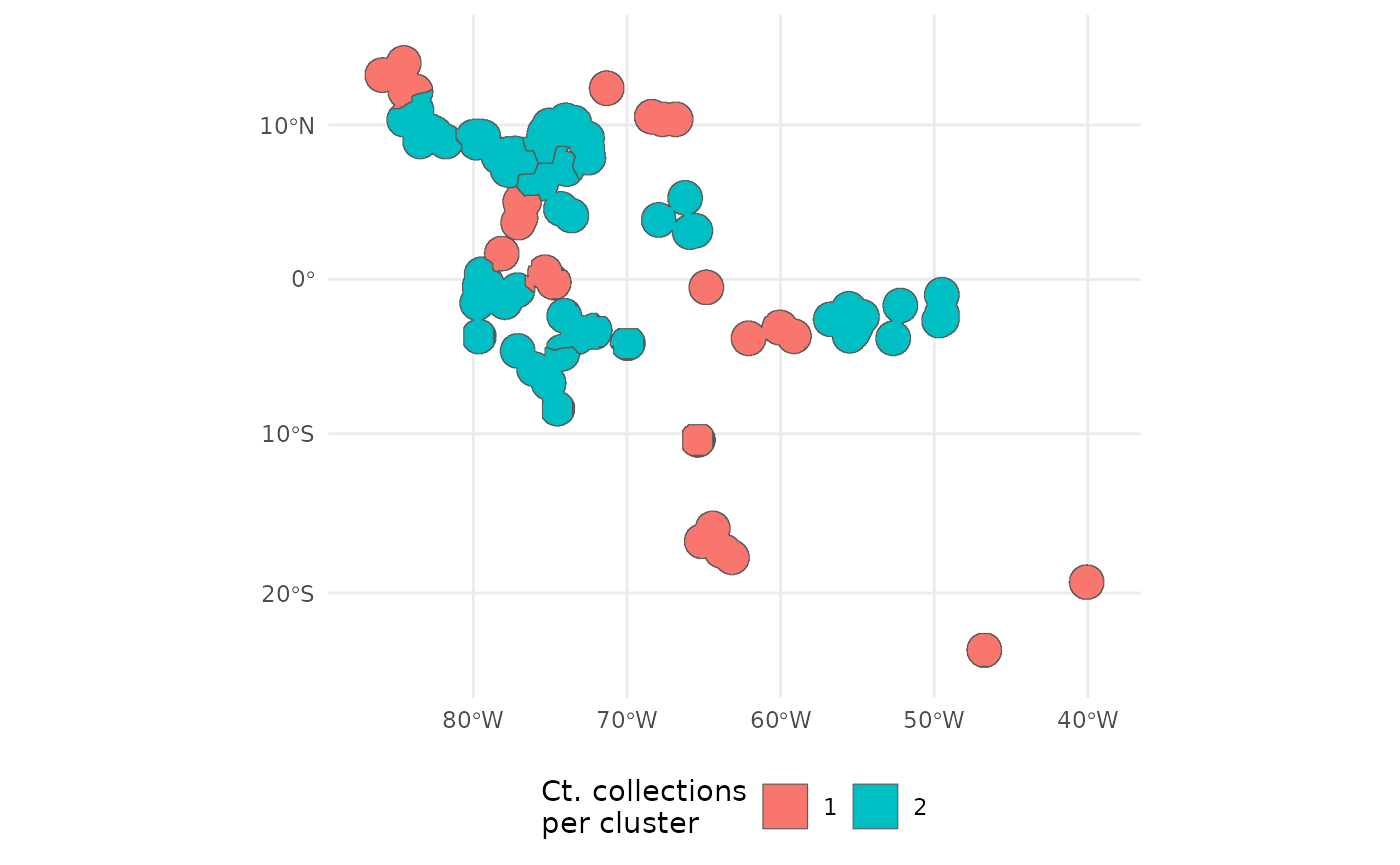
Each cluster has a different number of the 20 assigned collections.
bonus: adding sdm as a resistance layer, and non-linear scaling.
A default argument to cluster IBR is the probability surface predictions from an SDM. Here we will add it to the surface.
We will also show another way to add the topographic ruggedness index that bypasses the assumed linear relationship in the weighting scheme.
sdm <- terra::rast(
  file.path(system.file(package="safeHavens"), 'extdata',  'SDM_thresholds.tif')
  )
plot(sdm['Predictions'])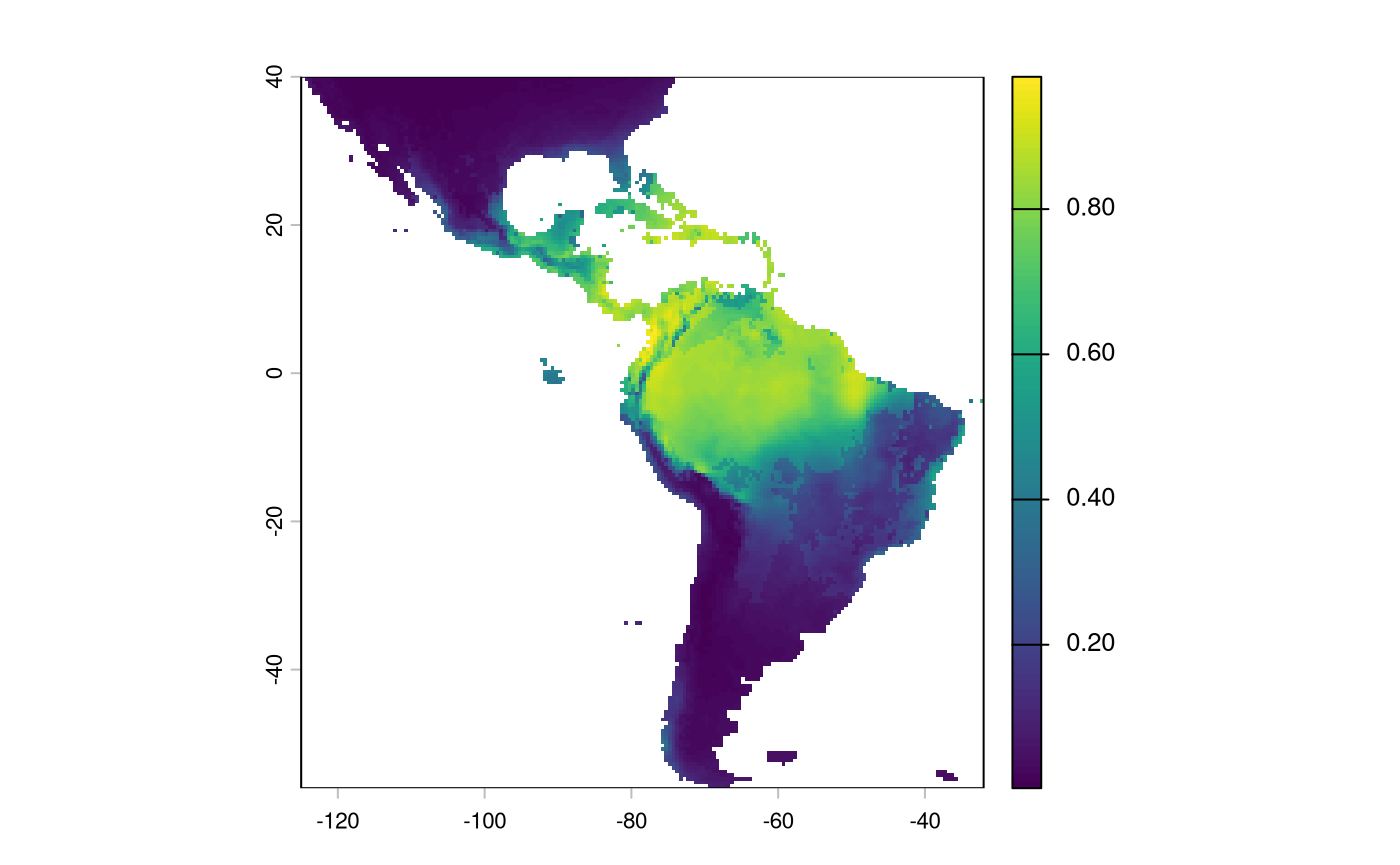
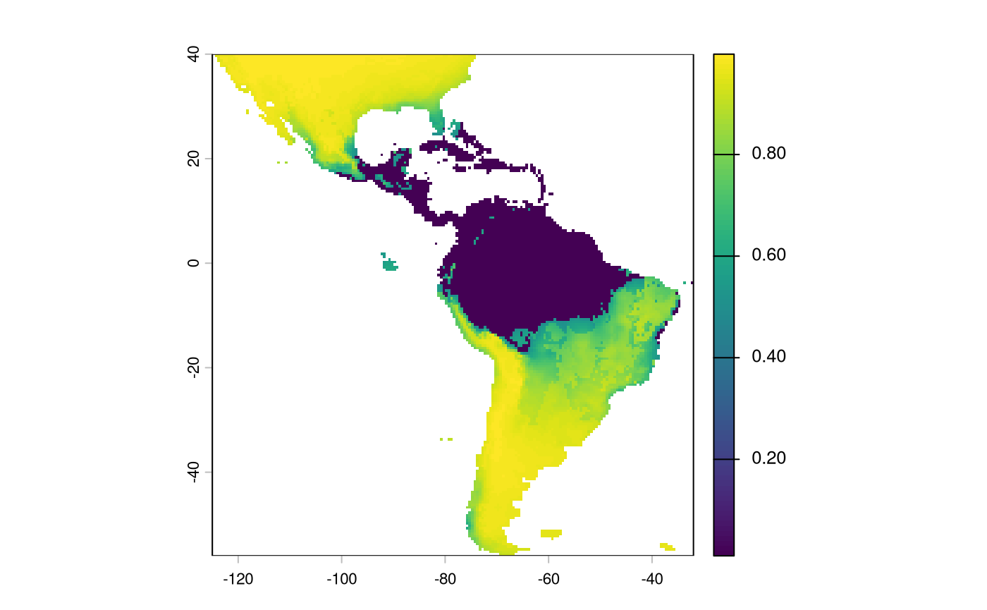
We will have to reverse the predictions from this layer; currently, higher values indicate a more suitable habitat. We want higher values in the probability surface function to indicate greater resistance to movement.
inverted_sdm <- 1 - sdm['Predictions']
plot(inverted_sdm)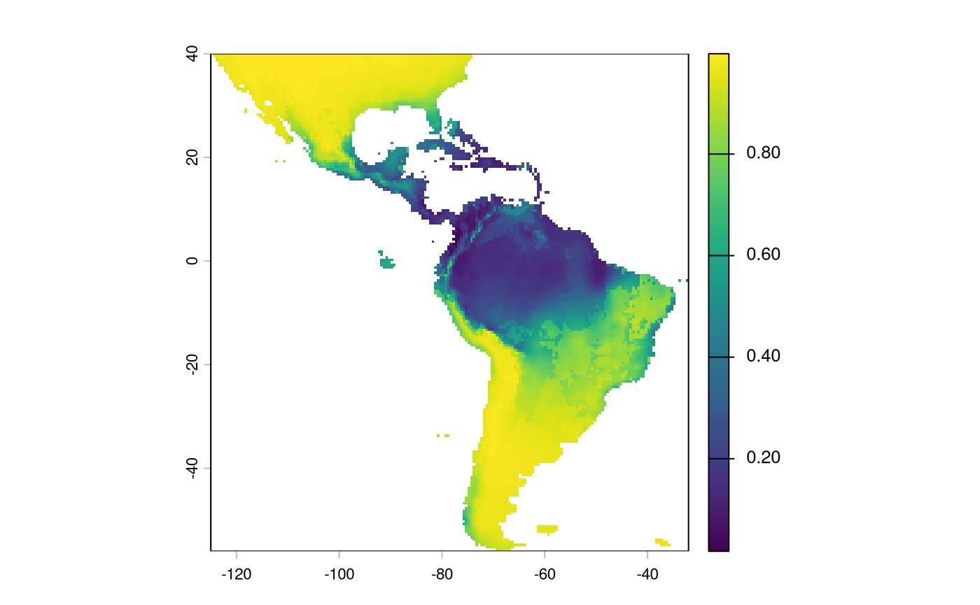
And indeed, we may actually just want to remove weights in a suitable habitat, or set them to an arbitrarily low value.
And we will convert it to the same integer scale as the other predictors.

Note that we will have to make sure our SDM aligns with the existing layers
inverted_sdm <- crop(inverted_sdm, ocean_r)
inverted_sdm <- resample(inverted_sdm, ocean_r)
inverted_sdm[is.na(inverted_sdm)] <- 99

plot(inverted_sdm)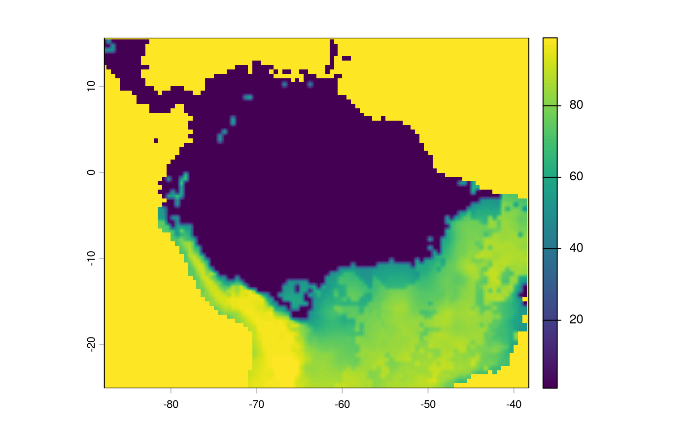
non-linear weight
Not all environmental variables are expected to have linear effects on movement. Indeed, something like terrain ruggedness may have only a small effect until reaching an asymptote.
x <- 1:100
rs <- function(x, to = c(0, 100)) {
  rng <- range(x, na.rm = TRUE)
  to[1] + (x - rng[1]) / diff(rng) * diff(to)
}

# display some transformations.
par(mfrow = c(2, 3), mar = c(4, 4, 2, 1))
plot(x, rs(sqrt(x)), type = "l", main = "sqrt(x)")
plot(x, rs(log1p(x)), type = "l", main = "log1p(x)")
plot(x, rs(asinh(x)), type = "l", main = "asinh(x)")
plot(x, rs(x^2), type = "l", main = "x^2: polynomial")
plot(x, rs(x^3), type = "l", main = "x^3: polynomial")
plot(x, rs(x^4), type = "l", main = "x^4 polynomial")![]()
We will apply a fourth-order polynomial to the input tri data to accommodate a non-linear effect.
tri_rscl <- app(tri, function(x) { rs(x^2, to = c(1, 80)) })

par(mfrow = c(1, 2), mar = c(4, 4, 2, 1))
plot(tri, main = 'Original')
plot(tri_rscl, main = 'Rescaled')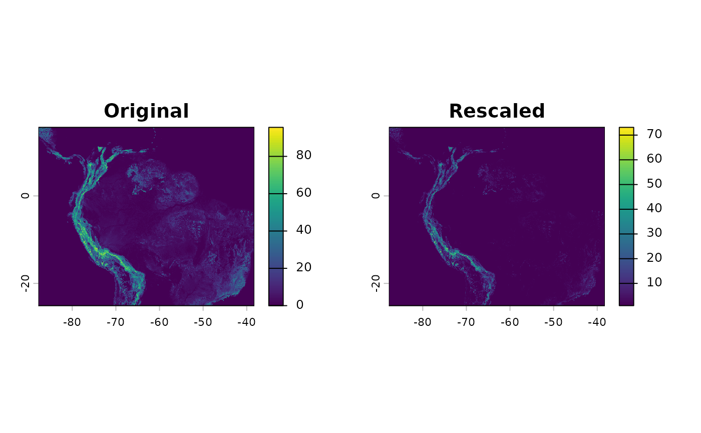
And we can create a new resistance surface
res_surface <- buildResistanceSurface(

  base_raster = rast(ocean_r), # template

  oceans = ocean_r, # rasters
  lakes = lakes_r,
  rivers = rivers_r,
  #tri = tri, # dont use me! i rescale.
  habitat = inverted_sdm,
  addtl_r = tri_rscl,

  w_ocean = 120, # weights to multiple  input raster values by --
  w_lakes = 70, # is 1 * 50
  w_rivers = 40, # is 1 *20
  w_habitat = 0.5,
  #w_tri = 4 # don't use me! use addtl_wt
  addtl_w = 1
)
par(mfrow=c(1,1))
plot(res_surface)