
Species Distribution Modelling
Before proceeding, please refer to all other vignettes, as they provide valuable foundational context, that will not be covered here. While the rationale here is roughly the same to the ‘Species Distribution Modelling’ and ‘Predictive Provenance’ vignettes, this approach focuses on improved uncertainty estimation during processing.
Background
This vignette details the steps required to create a Bayesian Species
Distribution Model (SDM) using functions from safeHavens,
which serve as wrappers for brms::brms(). Building on the foundational
rationale mentioned previously, the following information guides you
through the Bayesian-specific setup. The SDM raster surface is then
post-processed to create a binary raster map of suitable and unsuitable
habitat, which is used to rescale the environmental predictor variables
based on the SDM statistical models parameter posteriors. These
parameter posteriors are then used in a clustering algorithm to
partition the species range into more environmentallly similar regions
for germplasm sampling.
The goal of most SDMs is to create a model that accurately predicts where a species will be located in environmental space and can then be predicted in geographic space. The goal of these models is to understand the degree and direction to which various environmental features correlate with a species’ observed range.
About
In this section, we use Bayesian hierarchical models to model both the probability of suitable habitat for the species and paramter (indepdent variables) uncertainty of each variables contribution to the model. This enables clustering climatically similar areas using an SDM approach, linking the previously described methodology to specific analytical outcomes.
prep data
The data preparation steps described below are also found at the start of the ‘Predictive Provenance’ vignette. Recall these foundational steps as we transition into Bayesian-specific applications. To keep this vignette concise, some intermediate processing steps will be ‘hidden.’ This ensures the focus remains on the distinct Bayesian approach discussed in the sections above.
library(safeHavens)
library(sf) ## vector operations
library(terra) ## raster operations
library(geodata) ## environmental variables
library(dplyr) ## general data handling
library(tidyr) ## general data handling
library(ggplot2) ## plotting
library(patchwork) ## multiplots
library(pROC) ## for AUC and ROC curve plots
library(DHARMa) ## model resiudals
library(tidybayes) ## various posterior plots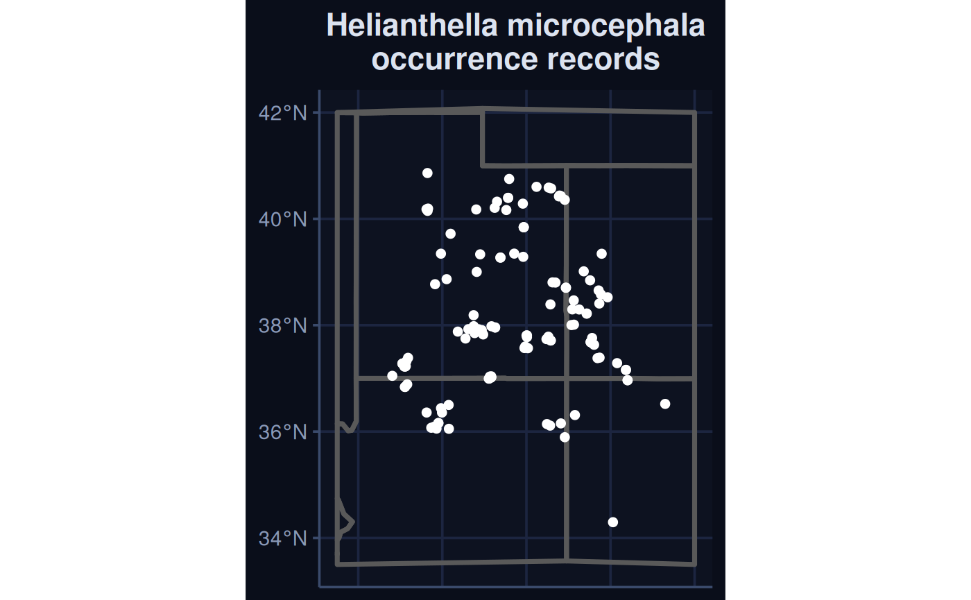
fit the model
Here we fit as SDM using bayesianSDM. For arguments, it
requires occurrence data x, a raster stack of
predictors, a quantile_v offset used to create
pseudo-absence data, and a planar_proj used to calculate
distances between occurrence data and possible pseudo-absence
points.
sdModel <- bayesianSDM(
  x = hemi,
  pca_predictors = FALSE,
  predictors = bio_current,
  quantile_v = 0.025,
  planar_proj = 5070,
  resample = TRUE,
  feature_selection = 'ffs',
  min_ffs_var = 3,
  fact = 3,
  silent = 2 # print fewer messages during model fit.
  )
Load a run of the model described above for the sake of this vignettes processing speed.
sdModel <- readRDS(
  file.path(system.file(package="safeHavens"), 'extdata',  'BayesSDM.rds')
  )

coefs <- rownames(as.data.frame(brms::fixef(sdModel$Model, summary = TRUE)))
sdModel$Predictors <- bio_current[[ coefs[grep('bio_', coefs)]]]

# add the above back on, had to save memory
sdModel$RasterPredictions <- terra::unwrap(sdModel$RasterPredictions)
sdModel$RasterPredictions_sd <- terra::unwrap(sdModel$RasterPredictions_sd)
sdModel$AOA <- terra::unwrap(sdModel$AOA)
Under the hood, this function uses brms, which
dispatches to Stan, to fit a Bayesian hierarchical model (GLMM), where
the distances between occurrence records are treated as fixed effects to
reduce the effects of spatial autocorrelation and increase the
interpretability of the model’s parameters.
explore the output
Plot the predictions
sdm_td <- sdModel$TrainData

par(mfrow = c(1, 2))
plot(sdModel$RasterPredictions, main = 'mean prediction')
points(vect(sdm_td[sdm_td$occurrence==1,]),col = 'black', cex = 0.5)
points(vect(sdm_td[sdm_td$occurrence==0,]),col = 'red', cex = 0.5)

plot(sdModel$RasterPredictions_sd, main = 'sd prediction')
points(vect(sdm_td[sdm_td$occurrence==1,]),col = 'black', cex = 0.5)
points(vect(sdm_td[sdm_td$occurrence==0,]),col = 'red', cex = 0.5)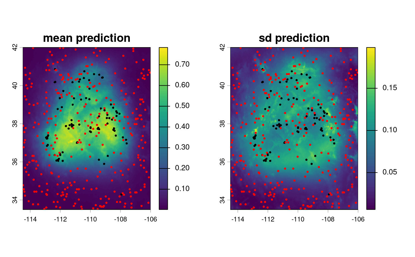
The brms:: model summary can be accessed from the sdModel list.
sdModel$Model
Warning: There were 32 divergent transitions after warmup. Increasing
adapt_delta above 0.99 may help. See
http://mc-stan.org/misc/warnings.html#divergent-transitions-after-warmup
 Family: bernoulli
  Links: mu = logit
Formula: occurrence ~ bio_02 + bio_03 + bio_04 + bio_09 + bio_14 + s(gp_x, gp_y, bs = "gp", k = 50)
   Data: sf::st_drop_geometry(train) (Number of observations: 415)
  Draws: 4 chains, each with iter = 5000; warmup = 2000; thin = 1;
         total post-warmup draws = 12000

Smoothing Spline Hyperparameters:
                 Estimate Est.Error l-95% CI u-95% CI Rhat Bulk_ESS Tail_ESS
sds(sgp_xgp_y_1)  1076.12    420.52   479.08  2109.27 1.00     2349     4826

Regression Coefficients:
            Estimate Est.Error l-95% CI u-95% CI Rhat Bulk_ESS Tail_ESS
Intercept       5.15      7.15    -3.30    21.86 1.00     2420     5747
bio_02         -0.03      0.11    -0.32     0.09 1.00     5916     5747
bio_03         -0.06      0.10    -0.31     0.03 1.00     3753     6509
bio_04         -0.00      0.00    -0.02     0.00 1.00     2778     6755
bio_09          0.00      0.02    -0.03     0.05 1.00     9355     9702
bio_14         -0.05      0.06    -0.19     0.01 1.00     2793     7626
sgp_xgp_y_1    -0.00      0.25    -0.28     0.28 1.00    11289     7949
sgp_xgp_y_2    -0.01      0.26    -0.32     0.25 1.00    12436     8781

Draws were sampled using sample(hmc). For each parameter, Bulk_ESS
and Tail_ESS are effective sample size measures, and Rhat is the potential
scale reduction factor on split chains (at convergence, Rhat = 1).
rHat < 1.01 is ideal; < 1.05 is acceptable. Both ESS should be greater than 400; increase iterations to achieve this. Divergence of 0 is ideal; any divergence is a flag for a possibly misspecified model.
Diagnostics can be accessed from a list, and the stan website has some information on them here, as well as warnings (as may be depicted above) https://mc-stan.org/misc/warnings/
Similar to elasticSDM, we also have an area of
applicability and other surfaces from CAST.
plot(sdModel$AOA)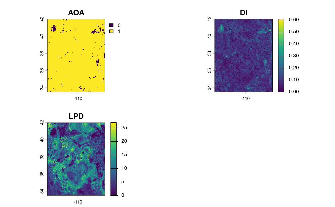
Diagnostics on the model come directly from Stan and brms::.
sdModel$Diagnostics
$max_Rhat
[1] 1.004849

$min_BulkESS
[1] 2131.685

$min_TailESS
[1] 4453.781

$n_divergent
[1] 32
To assess how well the model predicts the suitable habitat for the hold-out sample, the confusion matrix can be obtained from the test and train splits. While balanced accuracy for these is generally low, as these models are not intended for prediction, so much as understanding the relationships between environmental variables driving the species distribution, the results show the model was able to learn some important characteristics of the species.
knitr::kable(sdModel$ConfusionMatrix$byClass)| x | |
|---|---|
| Sensitivity | 0.5416667 |
| Specificity | 0.9102564 |
| Pos Pred Value | 0.6500000 |
| Neg Pred Value | 0.8658537 |
| Precision | 0.6500000 |
| Recall | 0.5416667 |
| F1 | 0.5909091 |
| Prevalence | 0.2352941 |
| Detection Rate | 0.1274510 |
| Detection Prevalence | 0.1960784 |
| Balanced Accuracy | 0.7259615 |
Observe how the selected model predicts the state of the test data. Note that these accuracy results are slightly higher than those from the CV folds. Understand that this is not a bug; CV folds test on their own holdouts, while this is a new holdout set. The main reason the confusion matrix results are likely to be higher is due to spatial autocorrelation, which is not addressed in a typical ‘random split’ of test and train data. Minimise the effects of spatial autocorrelation on the model by using CAST for spatially informed cross-validation.
Treat the CVStructure output as a more realistic assessment.
binarize the output
The Bayesian SDM is post-processed using the same
PostProcessSDM function as the elasticSDM workflow.
threshold_rasts <- PostProcessSDM(
  rast_cont = sdModel$RasterPredictions,
  test = sdModel$TestData,
  train = sdModel$TrainData,
  planar_proj = 5070,
  thresh_metric = 'equal_sens_spec',
  quant_amt = 0.2
  )
knitr::kable(threshold_rasts$Threshold)| kappa | spec_sens | no_omission | prevalence | equal_sens_spec | sensitivity | |
|---|---|---|---|---|---|---|
| thresholds | 0.220913 | 0.220913 | 0.0510473 | 0.2444197 | 0.2866278 | 0.2444197 |
We can compare the results of applying this function side by side using the function’s output.
terra::plot(threshold_rasts$FinalRasters)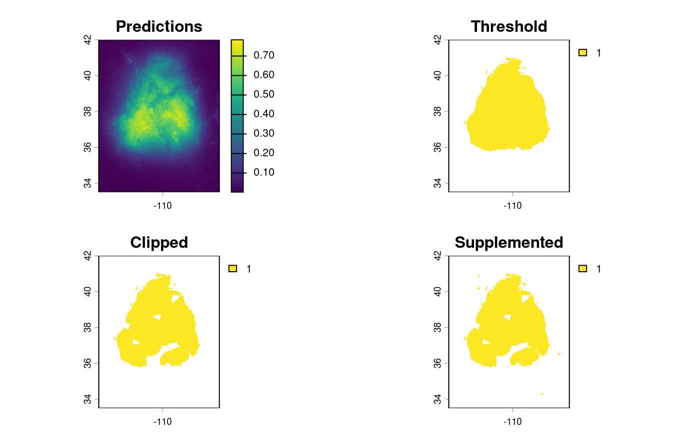
rescale predictor variables
The bayesianSDM requires a different function from
elasticSDM for creating weighted surfaces, with the suffix
RescaleRasters_bayes.
rr <- RescaleRasters_bayes(
  model = sdModel$Model,
  predictors = sdModel$Predictors,
  training_data = sdModel$TrainData,
  pred_mat = sdModel$PredictMatrix,
  include_uncertainty = TRUE
  )

terra::plot(rr$RescaledPredictors)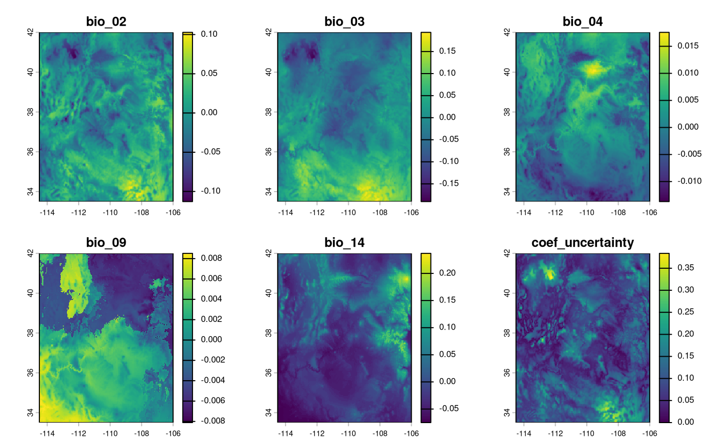
An optionally returned layer (via include_uncertainty =
TRUE) depicts areas with greater uncertainty towards the prediction.
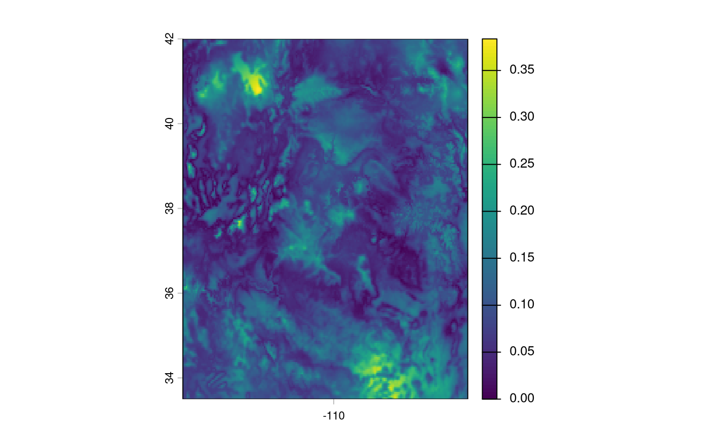
We can also show the variables that contributed the most to the sdm models’ predictions, along with their signs.
| Variable | Estimate | Est.Error | Q2.5 | Q97.5 | |
|---|---|---|---|---|---|
| 2 | bio_03 | -0.0597135 | 0.1015725 | -0.3129111 | 0.0253125 |
| 5 | bio_14 | -0.0481234 | 0.0588451 | -0.1918073 | 0.0109816 |
| 1 | bio_02 | -0.0287647 | 0.1124815 | -0.3225050 | 0.0859241 |
| 3 | bio_04 | -0.0047051 | 0.0048937 | -0.0158306 | 0.0014900 |
| 4 | bio_09 | 0.0041970 | 0.0163085 | -0.0253077 | 0.0466395 |
To delineate putative seed collection zones, we use the
PosteriorCluster function. It will use the raster surfaces
of the mean beta coefficient importance.
current_cluster <- PosteriorCluster(
  model = sdModel$Model,
  predictors = subset(rr$RescaledPredictors, 'coef_uncertainty', negate = TRUE),
  f_rasts = threshold_rasts$FinalRasters,
  lyr = 'Supplemented',
  pred_mat = sdModel$PredictMatrix,
  training_data = sdModel$Train,
  planar_proj = 5070,
  coord_wt = 0.5,
  n_pts = 5000
)
Drawing 100 posterior beta samples ...
Sampling fixed point set from prediction surface ...
  5000 of 5000 requested points have complete predictor data.
Computing habitat cost-distance MDS coordinates ...
Clustering over 100 posterior draws ...
  Draw 25 / 100
  Draw 50 / 100
  Draw 75 / 100
  Draw 100 / 100
Computing co-occurrence matrix ...
Deriving consensus clustering ...
  Consensus k = 20  [Hartigan = 20 (primary), CH = 4, Gamma = 20].
Computing top-3 cluster assignments per point ...
Projecting consensus clusters to raster ...
Loading required package: lattice
Using Bayesian posteriors and clustering allows us to identify areas with higher and lower uncertainty in clustering assignments. Areas with higher proportions had higher colocation scores than those with lower proportions.
plot(current_cluster$SummaryRaster$stability, main = 'Cluster Stability')
points(current_cluster$SamplePoints, cex = 0.1)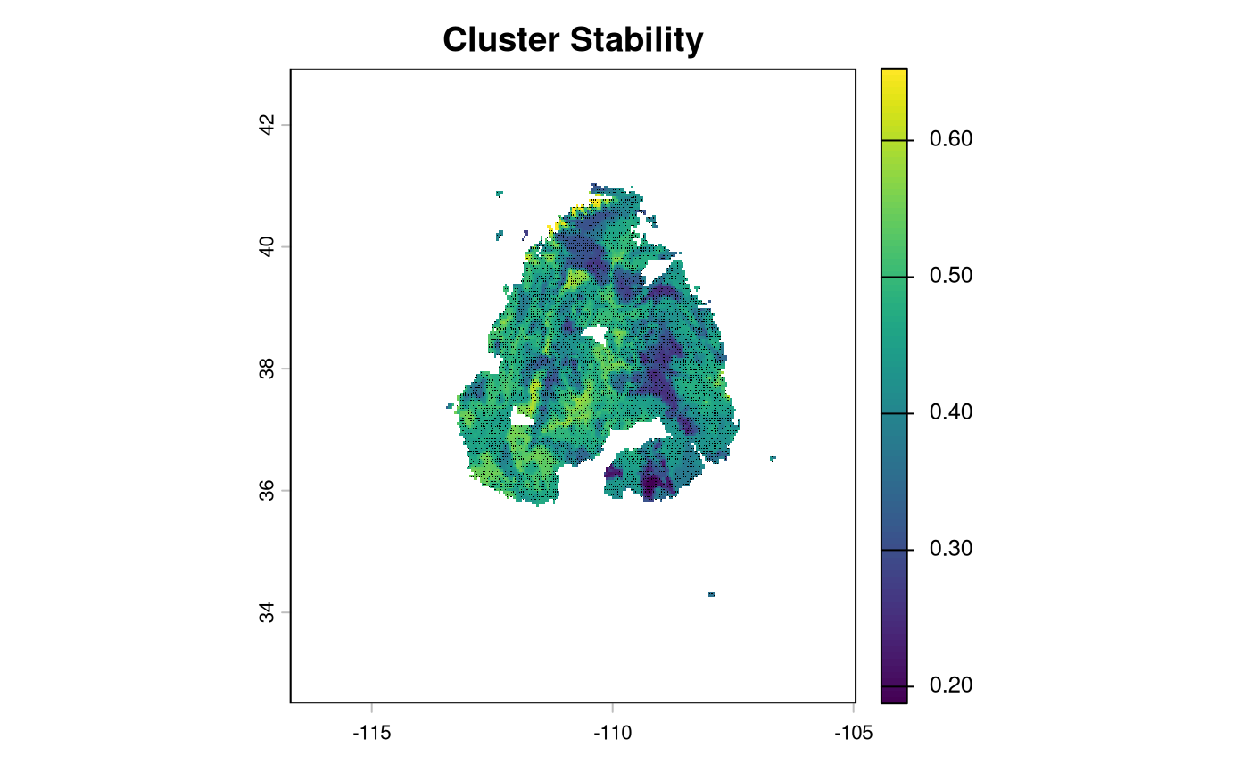
As with the other sampling functions, spatial polygons are returned for use with other applications.
bmap +
  geom_sf(data = current_cluster$Geometry, aes(fill = factor(ID))) +
  labs(fill = 'Cluster', title = 'Consensus Clusters')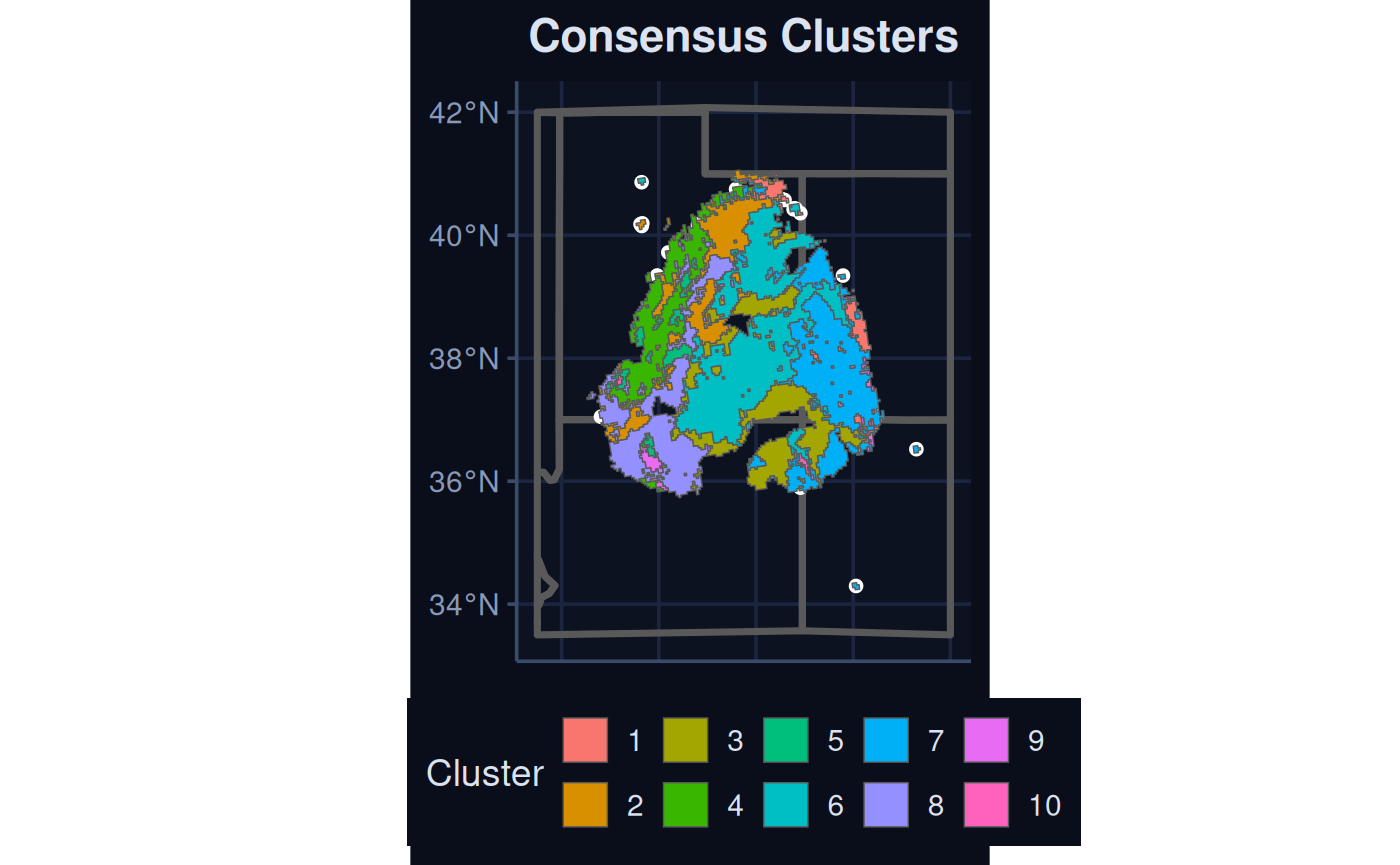
Interested users can see what the second-most and third-most stable clustering scenarios would look like via the following ranks. Do note that the renumbering of clusters from NW to SE (left to right, as many language groups read books) has not yet occurred on these rasters, so the numbers differ from the consensus surface.
par(mfrow = c(1, 3))
plot(as.factor(current_cluster$SummaryRaster$consensus), main = 'Consensus')
plot(current_cluster$RankRaster$rank2_final, main = '2nd most')
plot(current_cluster$RankRaster$rank3_final, main = '3rd most')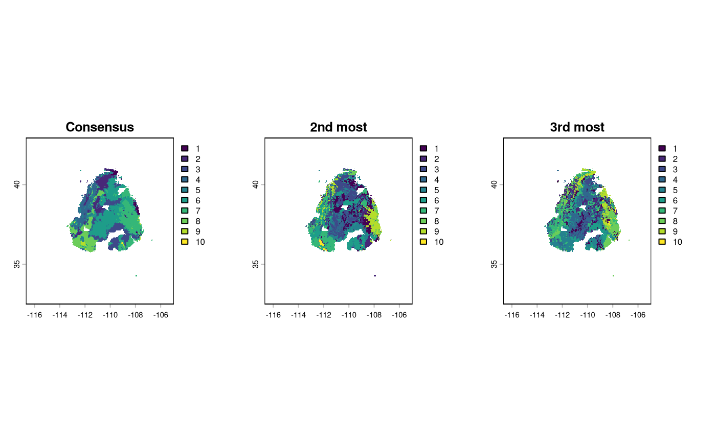
save results
writeSDMresults can also be used to save most of the core SDM output from the Bayesian workflow.
bp <- '~/Documents/assoRted/StrategizingGermplasmCollections'

writeSDMresults(
  cv_model = sdModel$CVStructure,
  model = sdModel$Model,
  cm = sdModel$ConfusionMatrix,
  coef_tab = rr$BetaCoefficients,
  f_rasts = threshold_rasts$FinalRasters,
  thresh = threshold_rasts$Threshold,
  file.path(bp, 'results', 'SDM'), 'hemi_test')

# we can see that the files were placed here using this.
list.files( file.path(bp, 'results', 'SDM'), recursive = TRUE )
predictive provenance
Here we use the predictive provenance approach for future time climate scenarios.
future_rescaled <- projectClustersBayes(
  bSDM_object = sdModel,
  posterior_clusters = current_cluster,
  future_predictors = bio_future,
  current_predictors = bio_current,
  threshold_rasts = threshold_rasts,
  planar_proj = "epsg:5070",
)
Warning: [spatSample] fewer cells returned than requested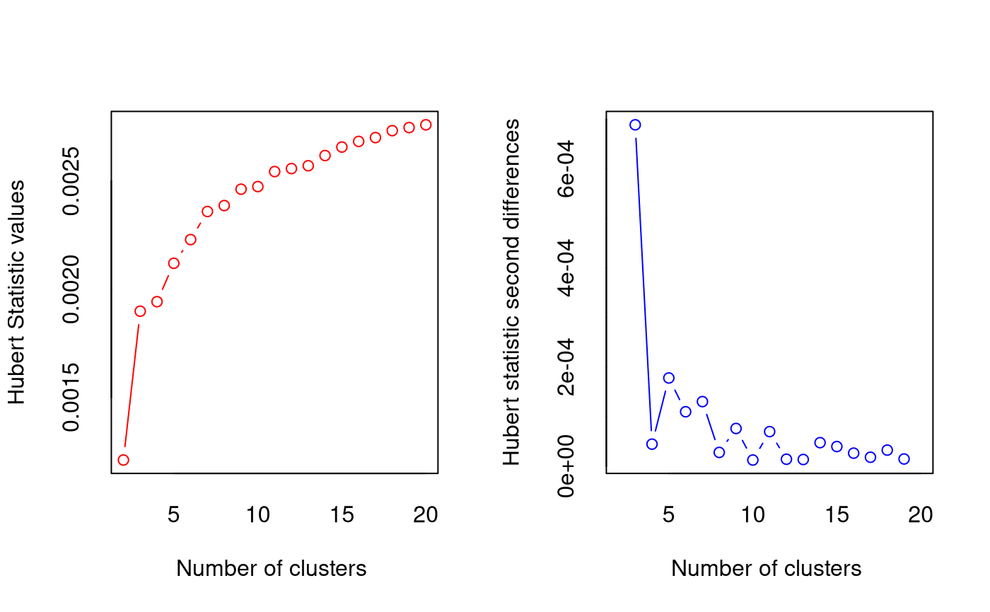
*** : The Hubert index is a graphical method of determining the number of clusters.
                In the plot of Hubert index, we seek a significant knee that corresponds to a
                significant increase of the value of the measure i.e the significant peak in Hubert
                index second differences plot.
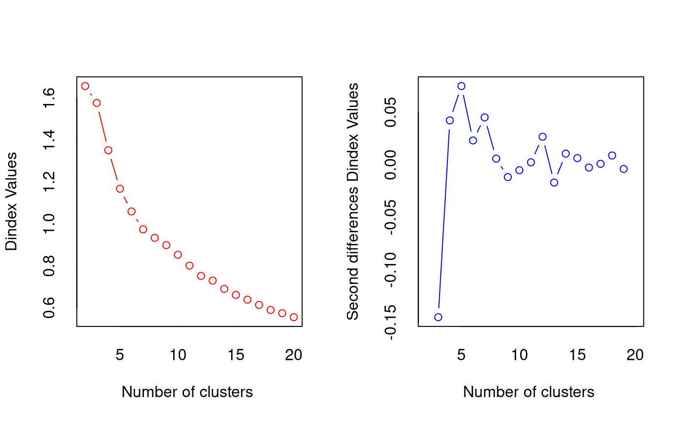
*** : The D index is a graphical method of determining the number of clusters.
                In the plot of D index, we seek a significant knee (the significant peak in Dindex
                second differences plot) that corresponds to a significant increase of the value of
                the measure.

*******************************************************************
* Among all indices:
* 4 proposed 2 as the best number of clusters
* 4 proposed 3 as the best number of clusters
* 10 proposed 4 as the best number of clusters
* 1 proposed 16 as the best number of clusters
* 1 proposed 18 as the best number of clusters
* 3 proposed 20 as the best number of clusters

                   ***** Conclusion *****

* According to the majority rule, the best number of clusters is  4


*******************************************************************
Warning: [spatSample] not all classes have 50 cells
We visualize the results for the current and future scenarios below.
nCl = seq(max(future_rescaled$Geometry$ID))
full_pal = c(
  '#a6cee3','#1f78b4','#b2df8a','#33a02c',
  '#fb9a99','#e31a1c','#fdbf6f','#ff7f00',
  '#cab2d6','#6a3d9a','#ffff99','#b15928'
  )
cus_pal <-full_pal[nCl]
names(cus_pal) <- nCl

bmap +
  geom_sf(
    data = current_cluster$Geometry,
    aes(fill = factor(ID),
    col = NA)
    ) +
  scale_fill_manual(values = cus_pal) +
  theme(legend.position = 'none', NULL) +
  labs(title = 'Current') +
bmap +
  geom_sf(
    data = future_rescaled$Geometry,
    aes(fill = factor(ID)),
    col = NA
    ) +
  scale_fill_manual(values = cus_pal) +
  labs(title = 'Future', fill = 'Cluster')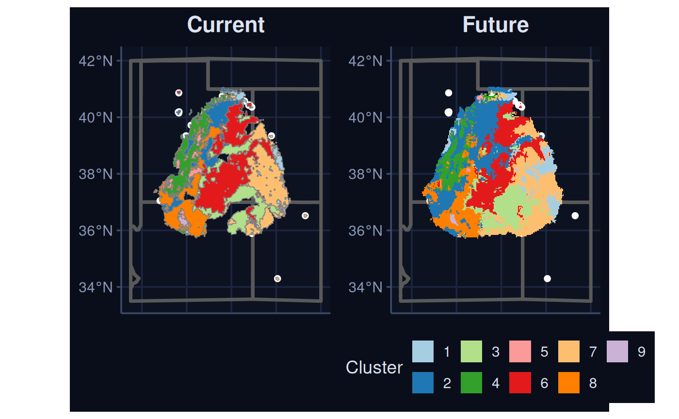
wrapping up
While the Bayesian hierarchical GLM does not produce excellent predictions of suitable habitat, it has several advantages. 1) It can incorporate spatial smoothers (splines) from mcgv to reduce the effects of spatial autocorrelation on model parameter estimates. 2) It provides uncertainty around the contribution of each selected predictor (i.e. many predictors can be weighed differently to get similar results).
bonus - model evaluation
The benefit of the bayesian approach, albeit at computational costs relative to the elasticNet workflow, are the estimates of uncertainty around the contributions of the independent variables towards predicting the species distribution. Both the predictive provenance workstreams rely heavily on ‘reading in’ to the contributions of independent variables that are correlated with the species distribution. We are excited to believe that many users will want to specify and iterate models to produce at least relatively robust models of species distributions.
Note that internally both the elastic and bayesianSDM functions perform a variety of operations to reduce the effects of spatial autocorrelation (spatial CV), pseudoreplication (spThin), and multicollinearity (VIF), on the interpretation of model coefficients. They further provide functionality to determine areas to which inference from the models can be made in geographic space in current times (AOA), and flag areas outside of known climate combinations in future scnearios (MESS).
In this section we briefly showcase a variety of model evaluation frameworks for understanding how performant models are. As this package essentially runs automated modelling processes, nearly all models could be improved upon manually by an analyst. However, given the scale of the biodiversity crisis, automated approaches are neccessary.
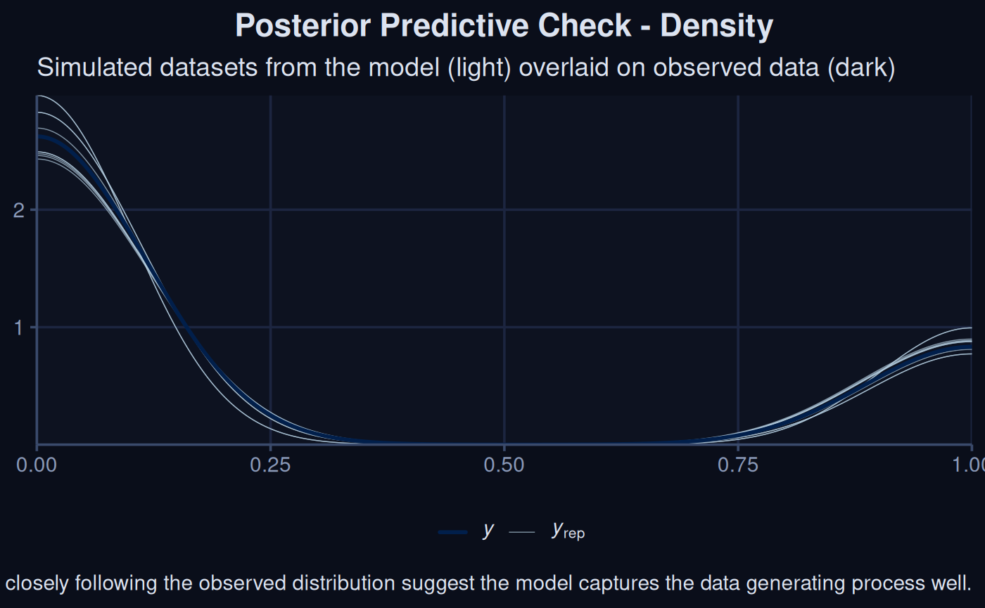
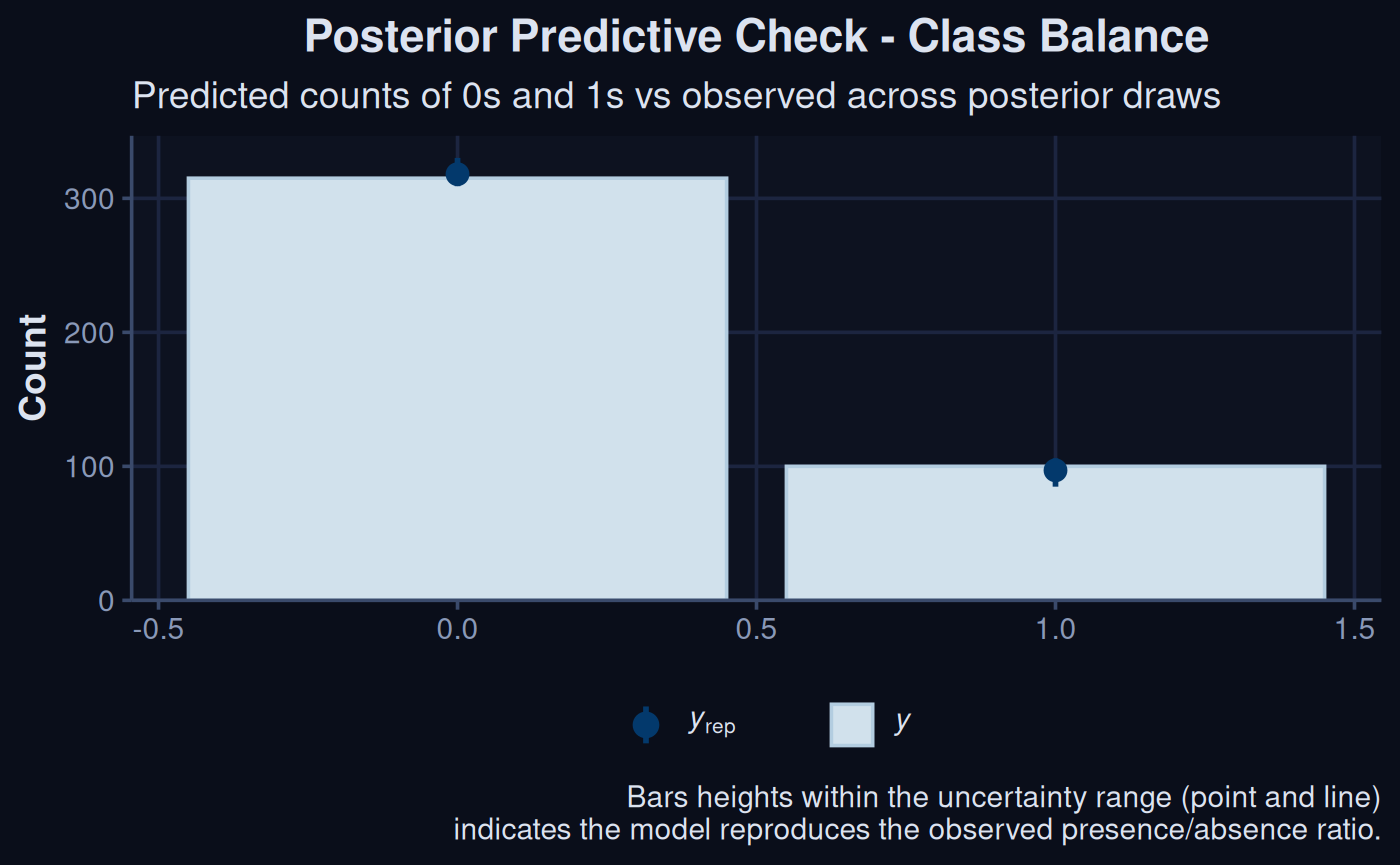
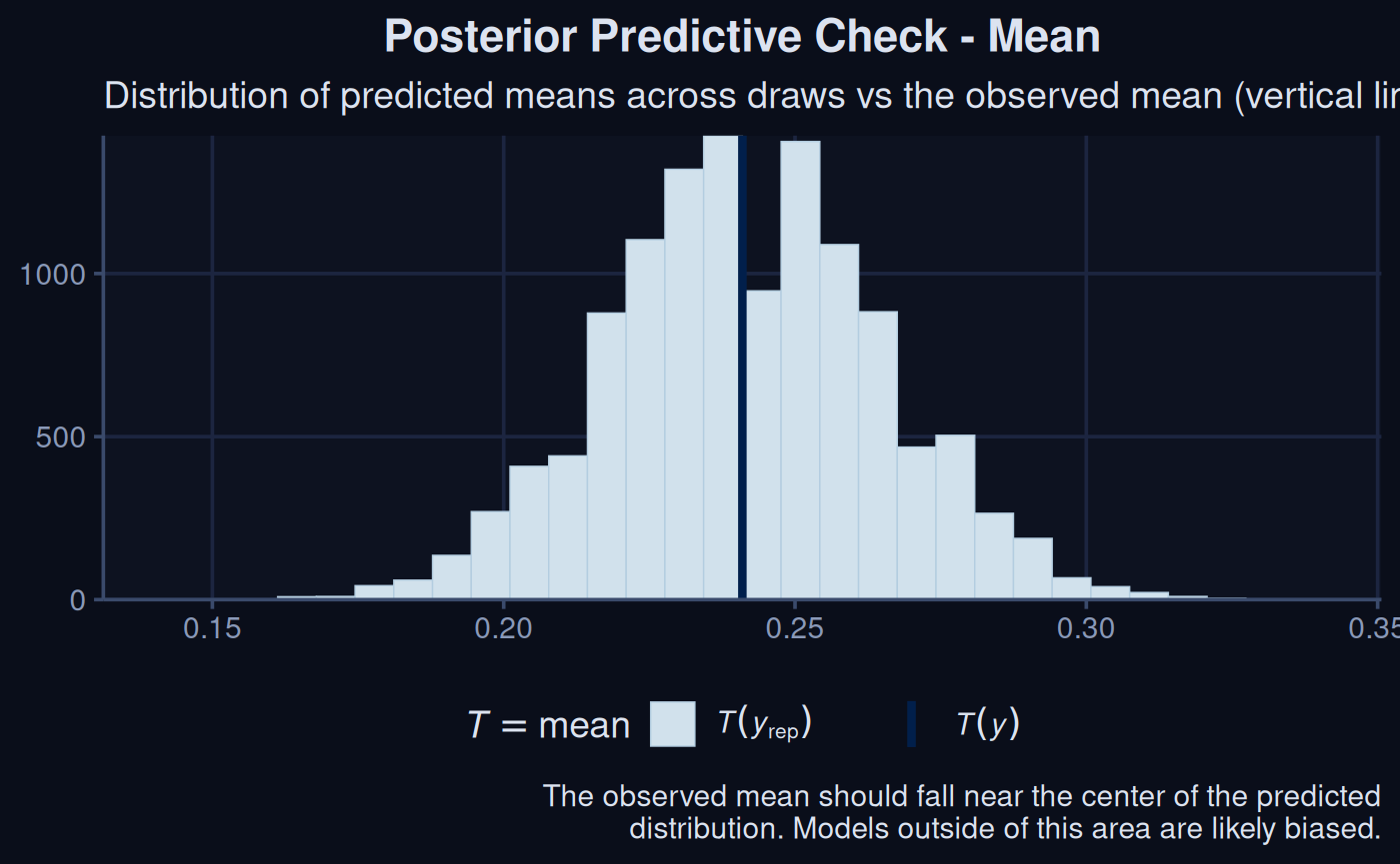
The following three plots all come directly from brms and versions for checking the posteriors predictions.
brms::pp_check(sdModel$Model, ndraws = 10) +
  labs(title = 'stuff') +
  theme_navy() +
  labs(
    title    = "Posterior Predictive Check - Density",
    subtitle = "Simulated datasets from the model (light) overlaid on observed data (dark)",
    caption  = "Lines closely following the observed distribution suggest the model captures the data generating process well."
) 
brms::pp_check(sdModel$Model, type = "bars", ndraws = 10) +
  labs(title = 'more') +
  theme_navy() +
  labs(
    title    = "Posterior Predictive Check - Class Balance",
    subtitle = "Predicted counts of 0s and 1s vs observed across posterior draws",
    caption  = "Bars heights within the uncertainty range (point and line)\nindicates the model reproduces the observed presence/absence ratio."
) 
brms::pp_check(sdModel$Model, type = "stat", stat = "mean") +
  labs(title = 'more') +
  theme_navy()  +
  labs(
    title    = "Posterior Predictive Check - Mean",
    subtitle = "Predicted means across draws vs the observed mean (vertical line)",
    caption  = "The observed mean should fall near the center of the predicted\ndistribution. Models outside of this area are likely biased."
) 
Areas of probability that the model has more difficulty predicting can also be visualized, using the method below. When the line deviates from the diagonal axis, it indicates a range of values they model is being overly or underconfident about assigning.
loo_probs <- tibble(
  pred_prob = brms::loo_epred(sdModel$Model, moment_match = TRUE)[, 1],
  observed  = factor(sdModel$TrainData$occurrence)
)
# Get posterior predicted probabilities
pred_probs <- sdModel$TrainData |>
  add_epred_draws(sdModel$Model, ndraws = 100) |>
  group_by(.row, .draw) |>
  summarise(prob = mean(.epred), .groups = "drop")
loo_probs |>
  mutate(bin = cut(pred_prob, breaks = 10)) |>
  group_by(bin) |>
  summarise(mean_pred = mean(pred_prob),
            mean_obs  = mean(as.numeric(as.character(observed)))) |>
  ggplot(aes(x = mean_pred, y = mean_obs)) +
  geom_point(col = '#dce3f0') +
  geom_line(col = '#dce3f0') +
  geom_abline(linetype = "dashed", col = '#dce3f0') +
  labs(
    x = "Mean LOO predicted probability",
    y = "Observed frequency",
    title    = "LOO Calibration",
    subtitle = "LOO predicted probabilities vs observed frequencies,\nbinned across the probability range",
    caption  = "Points close to the diagonal indicate well-calibrated predictions.\nDeviation suggests the model is over or underconfident in certain probability ranges."
    ) +
  theme_navy()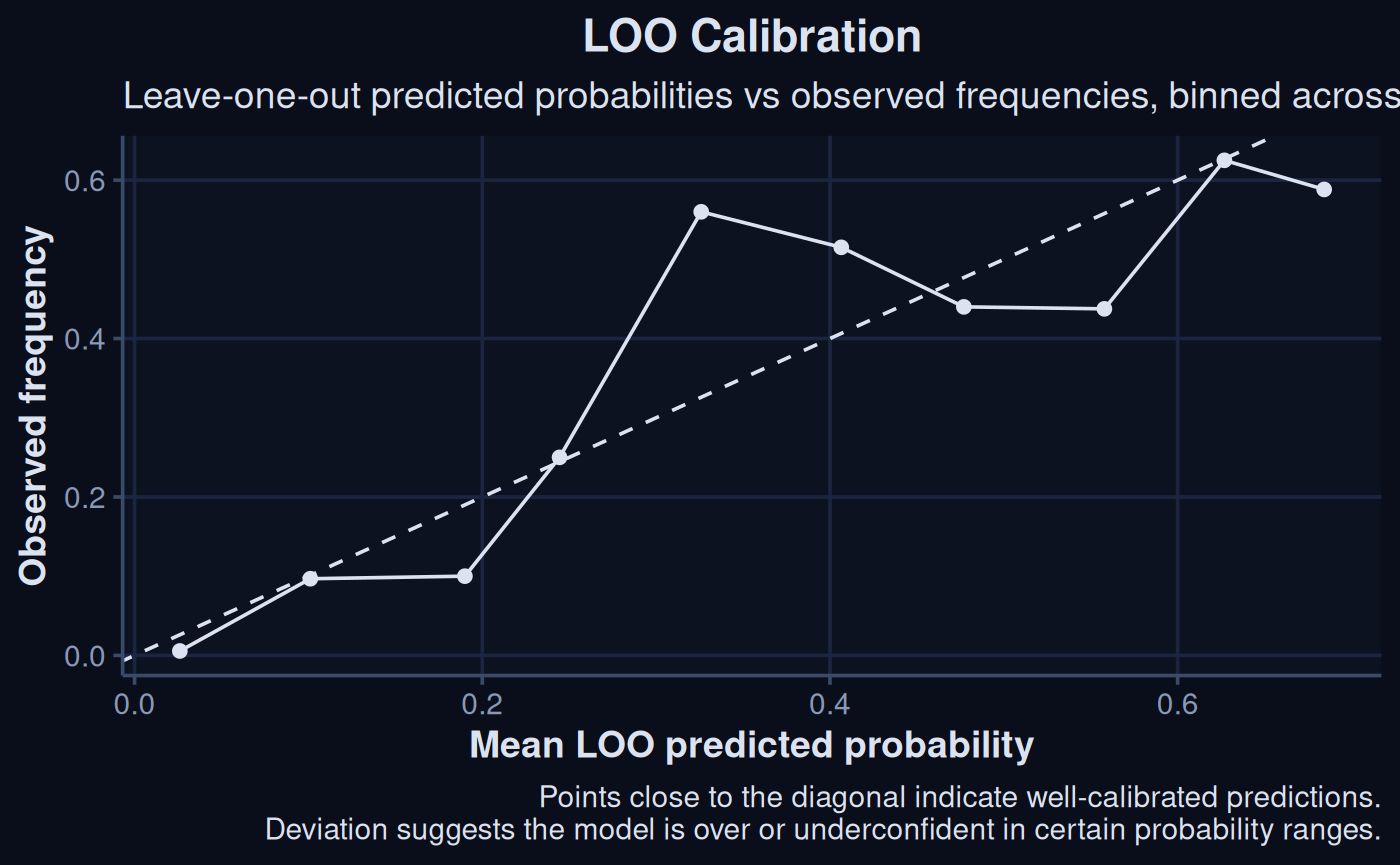
Bayesian methods allow for a posterior AUC distribution, these complement a mean point approach.
pred_probs |>
  group_by(.draw) |>
  summarise(
    auc = as.numeric(
      auc(
        roc(sdModel$TrainData$occurrence[.row],
        prob,
        quiet = TRUE))
        )
  ) |>
  ggplot(aes(x = auc)) +
  stat_halfeye(col = '#8B2635', fill = '#E0E2DB') +
  labs(
    x = "AUC",
    title    = "Posterior Distribution of AUC",
    subtitle = "Uncertainty in discrimination estimated from posterior\npredicted probabilities on training data",
    caption  = "AUC closer to 1 indicates better separation between presences and absences.\nThis is estimated on training data and will be optimistic use the matrix data from function."
) +
  theme_navy()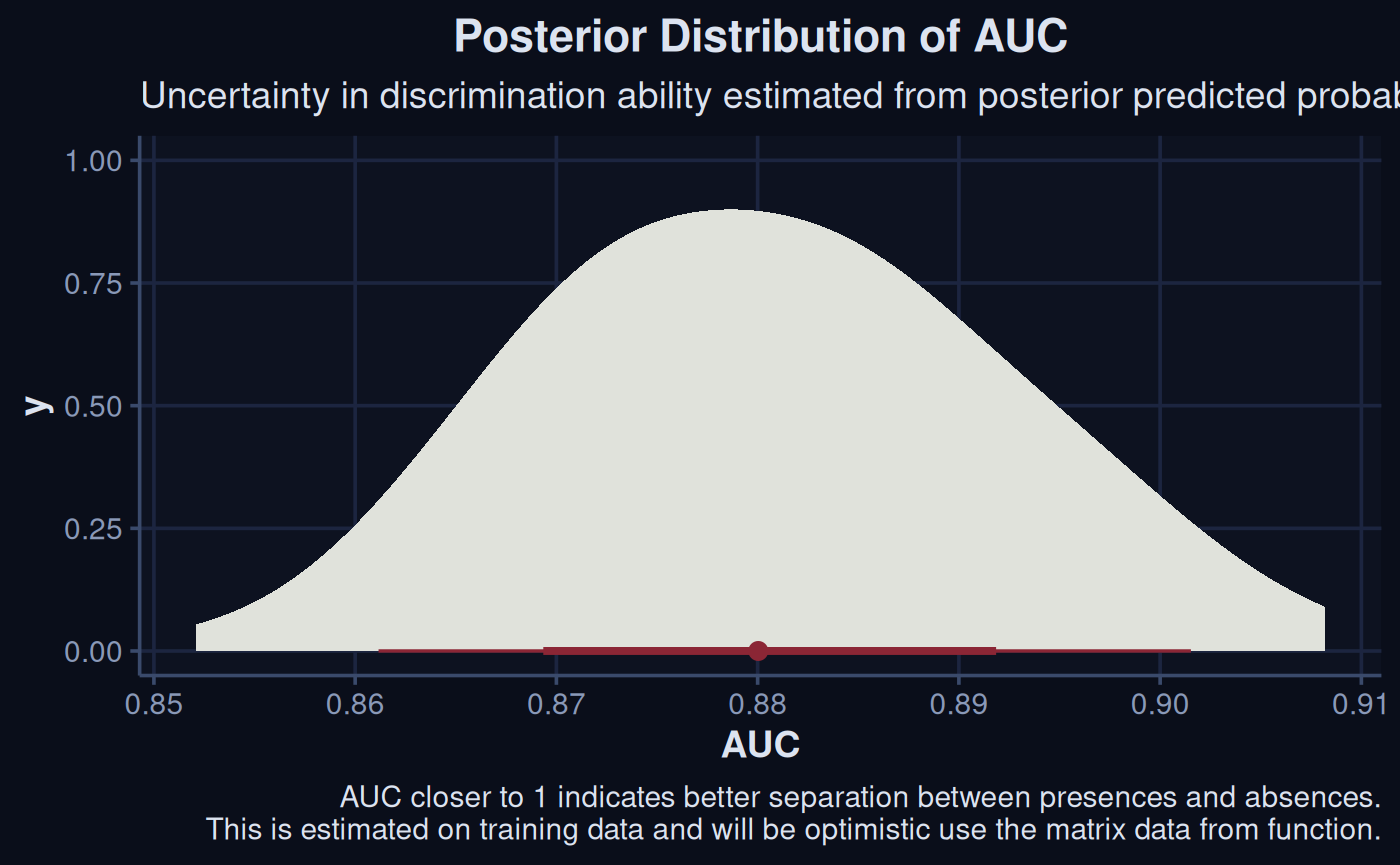
A simple receiver operator curve based on the LOO validation can be computed. These show the tradeoff in sensitivity and specificity across the models range.
update_geom_defaults("line",   list(colour = "#dce3f0"))
roc(loo_probs$observed, loo_probs$pred_prob) |>
  ggroc() +
  geom_abline(slope = 1, intercept = 1, linetype = "dashed", col = "#dce3f0") +
  labs(
    title    = "Leave-One-Out ROC Curve",
    subtitle = "ROC curve using LOO predicted probabilities",
    caption  = "The curve shows the tradeoff between true positive and false positive rates\nacross all classification thresholds.\nCurves closer to the top-left corner indicate strong out-of-sample discrimination."
  ) +
  theme_navy()
Setting levels: control = 0, case = 1
Setting direction: controls < cases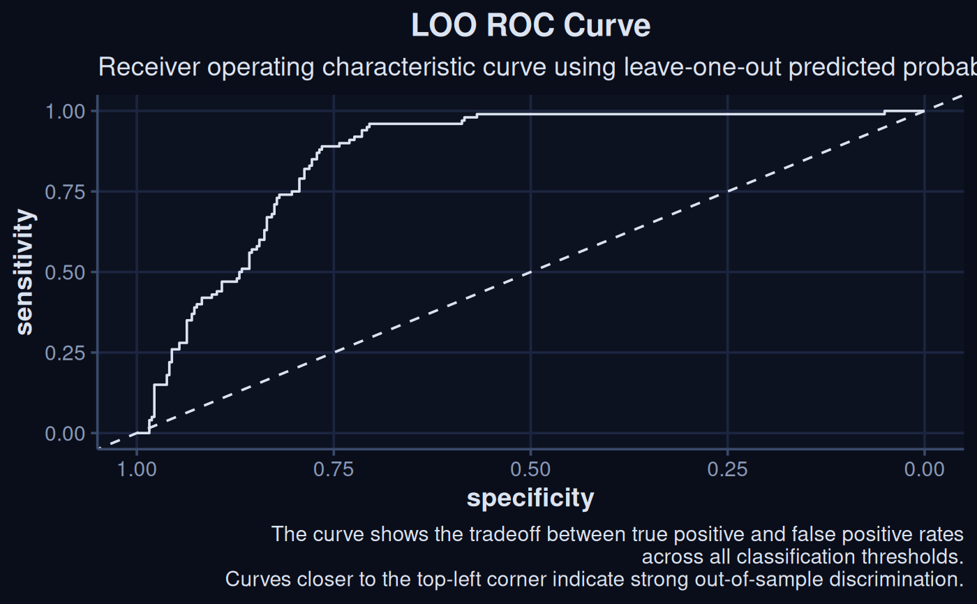
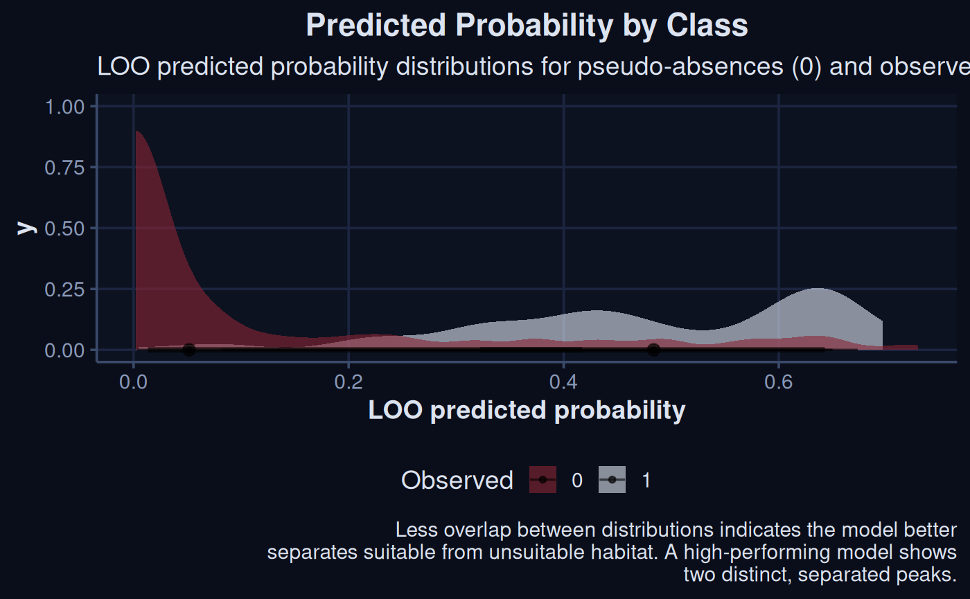
The ability for the model to discrimate between categorical classes,
such as from a bernoulli model, can be visualized as well. In the
following plot perfectly separated densities would indicate a model with
perfect discrimination. The plot below will roughly tie into the ideas
behind the threshold metrics used in PostProcessSDM.
loo_probs |>
  ggplot(aes(x = pred_prob, fill = observed)) +
  stat_halfeye(alpha = 0.6) +
  scale_fill_manual(values = c('#8B2635', '#dce3f0')) +
  labs(x = "LOO predicted probability", fill = "Observed") +
  theme_navy() +
  labs(
    title    = "Predicted Probability by Class",
    subtitle = "LOO predicted probability distributions for pseudo-absences (0) and presences (1)",
    caption  = "Less overlap between distributions indicates the model better\nseparates suitable from unsuitable habitat. A high-performing model shows\ntwo distinct, separated peaks."
    )
We can also check model residuals after transformation to determine if assumptions of indepdenence of individual errors are violated using DHARMa.
sims <- brms::posterior_predict(sdModel$Model, ndraws = 500)

dharma_res <- createDHARMa(
  simulatedResponse = t(sims),
  observedResponse  = sdModel$TrainData$occurrence,
  fittedPredictedResponse = apply(sims, 2, mean)
)

plot(dharma_res)# QQ + residuals vs fitted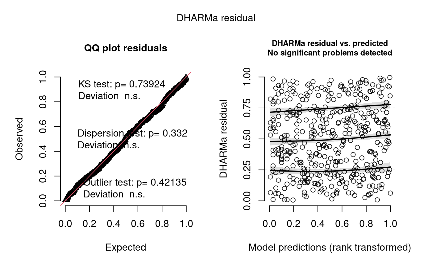
We can see the simulated posterior effect of each predictor on the models outcome.
spr_draw <- sdModel$Model |>
  spread_draws(`b_.*`, regex = TRUE) |>
  select(starts_with('b_bio'))

spr_draw |>
  pivot_longer(starts_with("b_"), names_to = "param", values_to = "value") |>
  ggplot(aes(x = value)) +
  stat_dots(alpha = 0.7, normalize = "panels") +
  facet_wrap(~ param) +
  theme(legend.position = "none") +
  theme_navy() +
  labs(
    title    = "Posterior Distribution per Predictor",
    subtitle = "Each panel shows the full posterior sample of a predictor's coefficient on its own scale",
    caption  = "Wider distributions indicate greater uncertainty in a variable's effect.\nDistributions overlapping zero suggest weaker or less certain contributions to the model."
  )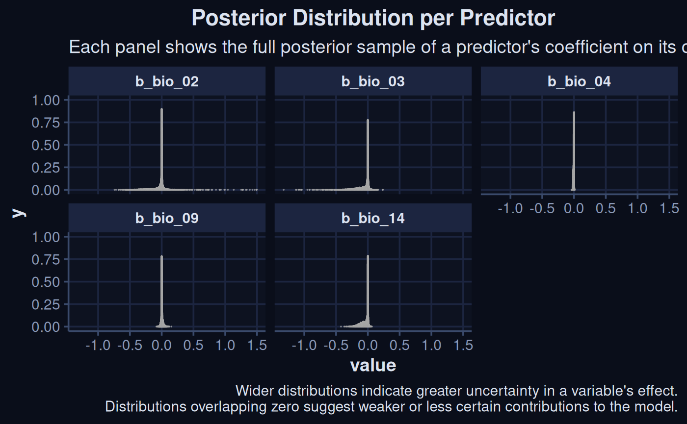
The posterior distribution of each predictor is shown above. The widths show the uncertainty around the effect of each variable on the species distribution.
spr_draw |>
  mutate(across(everything(), scale)) |>
  pivot_longer(
    everything(),
    names_to = "param",
    names_transform = list(param = \(x) sub("^b_", "", x)),
    values_to = "value"
  )|>
  ggplot(aes(x = value, y = reorder(param, value))) +
  stat_halfeye(col = '#8B2635', fill = '#9191E9') +
  xlim(-5, 5) + ## tighten this up for visualizing on vignette html page
  geom_vline(xintercept = 0, linetype = "dashed", col = '#E0E2DB') +
  labs(
    x = "Posterior estimate",
    y = NULL,
    title    = "Standardised Posterior Effects",
    subtitle = "Predictor coefficients scaled to unit variance, allowing direct comparison of effect sizes",
    caption  = "Variables further from zero have stronger effects on predicted occurrence.\nTighter distributions indicate more certainty - wide distributions crossing zero warrant caution."
    ) +
theme_navy() 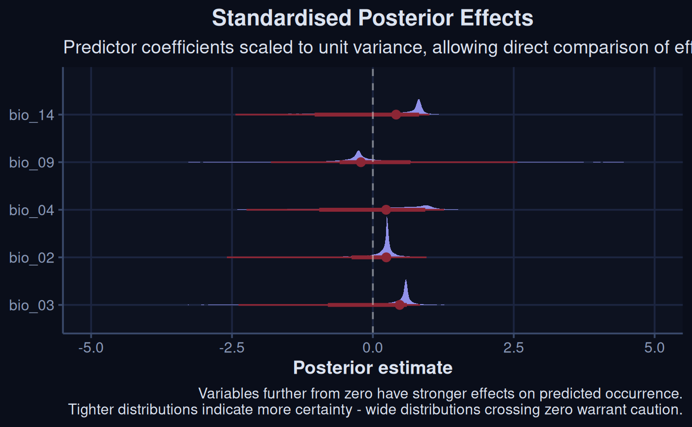
Variables with tighter density of predictions, and further from 0, have the largest effects on the outcome in the model.
plots <- purrr::map(
  gsub("^b_", '', colnames(spr_draw) ), ~
  marginaleffects::plot_predictions(sdModel$Model, condition = .x) +
    labs(title = .x) +
    xlab(NULL) +
    ylim(0,1) +
    theme_navy() +
    theme(legend.position = 'none') +
    ggplot2::update_geom_defaults("ribbon", list(fill = "#8b2635")) +
    ggplot2::update_geom_defaults("line", list(colour = "white"))
)

patchwork::wrap_plots(plots, ncol = 1) +
  plot_annotation(
    title    = "Marginal Effects per Predictor",
    subtitle = "Predicted occurrence probability across each variable's range,\naveraged over all other predictors",
    caption  = "The shape of each curve reveals whether a variable has a linear, threshold,\nor unimodal relationship with occurrence. Wider ribbons indicate greater uncertainty,\noften at the extremes of a variable's range."
) +
  plot_annotation(theme = theme(
    plot.background = element_rect(fill = "#0a0e1a", colour = NA),
    plot.title      = element_text(face = "bold", size = rel(1.2),colour = "#dce3f0"),
    plot.subtitle   = element_text(colour = "#dce3f0", size = rel(1.1)),
    plot.caption   = element_text(colour = "#dce3f0", size = rel(1))
  ))
Warning:
[1m
[22mUsing alpha for a discrete variable is not advised.

[1m
[22mUsing alpha for a discrete variable is not advised.

[1m
[22mUsing alpha for a discrete variable is not advised.

[1m
[22mUsing alpha for a discrete variable is not advised.

[1m
[22mUsing alpha for a discrete variable is not advised.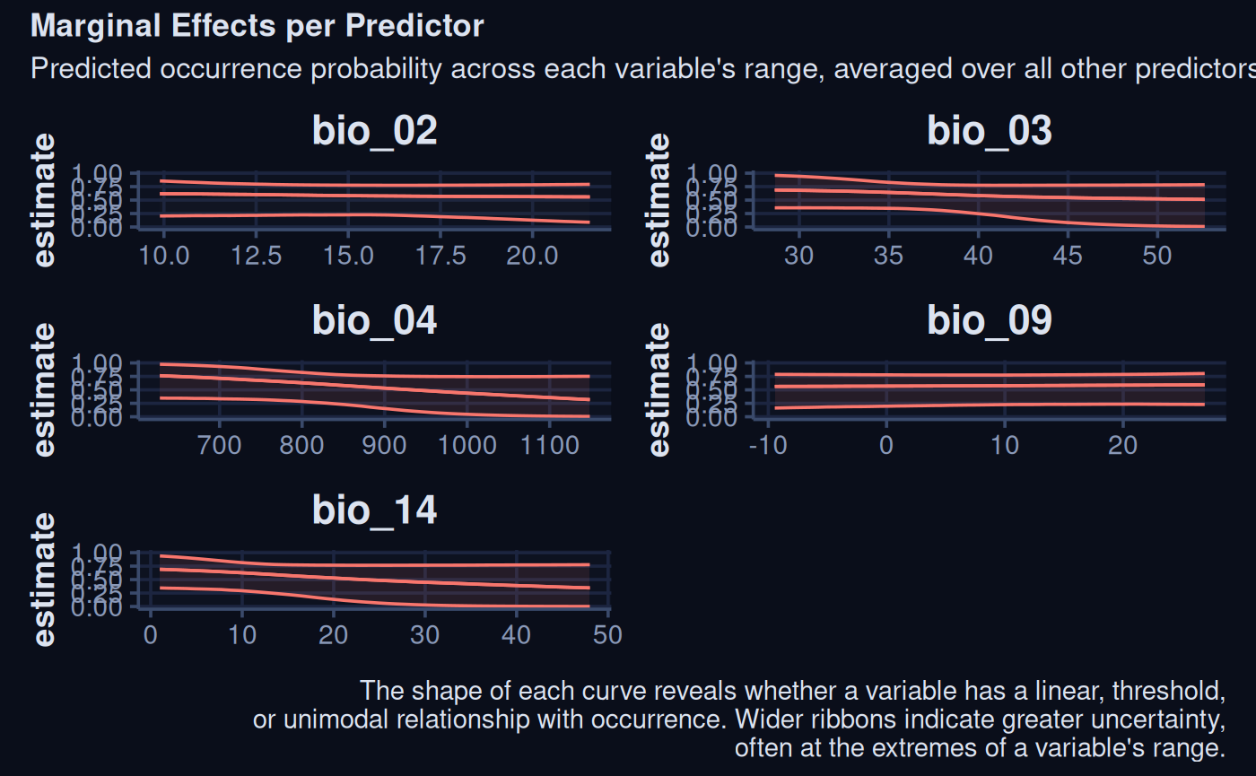
update_geom_defaults("line", list(colour = "black"))